Beam groups

For convenience, the BeamletOptics.AbstractBeamGroup offers a container-like interface for groups of Beams as commonly used in other software packages. The available beam groups are shown in the Beam catalog; the following sections describe the constructors that generate them.

Moving a beam group

Every beam group has a source position (center) and an orientation matrix, whose second column is the central source direction and whose first column is the sampling reference vector (basis). Both are updated when the group is moved. Refer to BeamletOptics.AbstractBeamGroup for the convention and to Moving sources for the kinematic API.

Center ray

The first beam of every CollimatedSource and PointSource generated by one of the constructors below is the center ray: it starts at the source position along the central source direction. This does not apply to sources that wrap given beams.

Collimated beam source

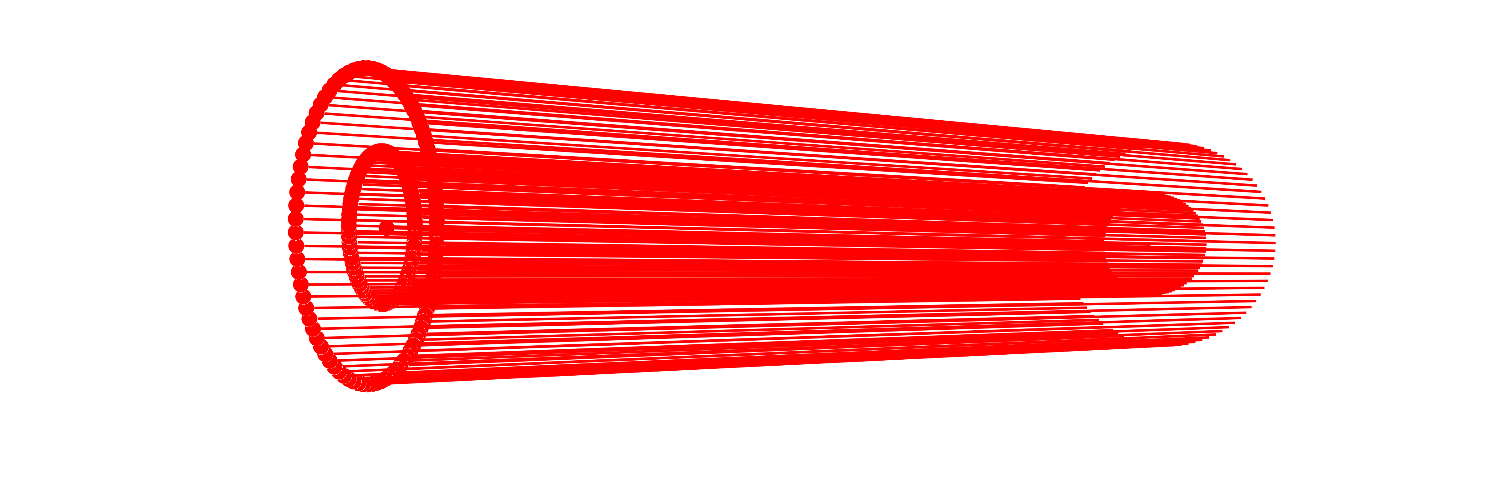
The collimated beam source is ideal to model light coming from a focal plane at infinity. This is useful for simulating plane wavefronts. You can define a collimated monochromatic Beam source as follows:

BeamletOptics.CollimatedSource Method

CollimatedSource(pos, dir, diameter, λ; num_rings, num_rays, basis)

Spawns a bundle of collimated Beams at the specified position and direction. The source is modelled as a ring of concentric beam rings around the center beam. The amount of beam rings between the center ray and outer diameter can be specified via num_rings.

Warning

For correct sampling, num_rays must be at least 20 times num_rings, otherwise an ArgumentError is thrown.

Arguments

The following inputs and arguments can be used to configure the CollimatedSource:

Inputs

• pos: center beam starting position

• dir: center beam starting direction

• diameter: outer beam bundle diameter in [m]

• λ = 1e-6: wavelength in [m], default val. is 1000 nm

Keyword Arguments

• num_rings: number of concentric beam rings, default is 10; the number of rings counts the center as the innermost one, i.e. num_rings - 1 rings lie around it

• num_rays: total number of rays in the source, default is 100x num_rings

• basis: Optional reference vector (e.g. [1,0,0]) to define the starting azimuthal angle for the beam rings.

Reproducible sampling

If no basis is passed, the orthogonal basis vectors spanning the pupil plane are derived from dir deterministically, so two sources sharing the same dir, diameter, num_rings and num_rays sample exactly the same ray positions. Pass a basis to rotate the azimuthal sampling of a source about its own axis, e.g. to interleave several otherwise identical sources.

source

Already existing beams, e.g. Beams of PolarizedRays as in the Vectorial focusing at high NA example, can be wrapped into a group with CollimatedSource(beams, diameter, pos, dir). PointSource(beams, NA, pos, dir) and AstigmaticBeamGroup(beams, pos, dir) work analogously; instead of dir, a full orientation matrix can be passed.

A special constructor called UniformDiscSource is available, which offers an equal-area sampling (Fibonacci pattern) and is thus favorable in situations where the weighting of the individual beams becomes important, e.g. for calculating a point spread function using the intensity function.

BeamletOptics.UniformDiscSource Function

UniformDiscSource(pos, dir, diameter, λ; num_rays=1_000, basis)

Generates a ray fan with equal area per ray across a circular pupil using the deterministic sunflower (Fibonacci) pattern.

The spiral starts with the center ray at pos (k = 0). The radius of the k-th ray (k = 1 … N-1) is ρₖ = diameter/2 ⋅ √((k + ½)/N), its azimuth is k times the golden angle π(3 - √5).

Note

This is merely a CollimatedSource constructor which uses Fibonacci sampling instead of concentric rings. All rays are equally weighted samples of the pupil: ray k represents the part of the disc between the radii diameter/2 ⋅ √(k/N) and diameter/2 ⋅ √((k + 1)/N). The center ray represents the innermost of these parts, a disc, by its center.

Arguments

The following inputs and arguments can be used to configure the underlying CollimatedSource:

Inputs

• pos: center of the pupil disc, i.e. the source position

• dir: starting direction of all beams

• diameter: outer beam bundle diameter in [m]

• λ = 1e-6: wavelength in [m]

Keyword Arguments

• num_rays=1000: total number of rays in the source, must be ≥ 1

• basis: Optional reference vector (e.g. [1,0,0]) to define the starting azimuthal angle of the sunflower pattern.

Reproducible sampling

If no basis is passed, the orthogonal basis vectors spanning the pupil plane are derived from dir deterministically, so two sources sharing the same dir, diameter and num_rays sample exactly the same ray positions. Pass a basis to rotate the sunflower pattern about its own axis, e.g. to interleave several otherwise identical sources.

source

Point beam source

The PointSource type is used to model emission from a spatially localized source that radiates Beams in a range of directions. This is commonly used to simulate conical emission patterns, such as light emerging from a fiber tip or a light source for a lens objective with a known focal distance. You can specify the origin and a propagation direction, which are then used to construct the monochromatic PointSource.

BeamletOptics.PointSource Method

PointSource(pos, dir, θ, λ; num_rings, num_rays, basis)

Spawns a point source of Beams at the specified position and direction. The point source is modelled as a collection of concentric beam fans centered around the center beam. The amount of beam rings between the center ray and half-spread-angle θ can be specified via num_rings.

Warning

For correct sampling, num_rays must be at least 20 times num_rings, otherwise an ArgumentError is thrown.

Arguments

The following inputs and arguments can be used to configure the PointSource:

Inputs

• pos: center beam starting position

• dir: center beam starting direction

• θ: half spread angle in rad, must be < π

• λ = 1e-6: wavelength in [m], default val. is 1000 nm

Keyword Arguments

• num_rings: number of concentric beam rings, default is 10; the number of rings counts the center as the innermost one, i.e. num_rings - 1 rings lie around it

• num_rays: total number of rays in the source, default is 100x num_rings

• basis: Optional reference vector (e.g. [1,0,0]) to define the starting azimuthal angle for the source rings.

Reproducible sampling

If no basis is passed, the orthogonal basis vectors are derived from dir deterministically, so two sources sharing the same dir, θ, num_rings and num_rays sample exactly the same ray directions. Pass a basis to rotate the azimuthal sampling of a source about its own axis, e.g. to interleave several otherwise identical sources.

source

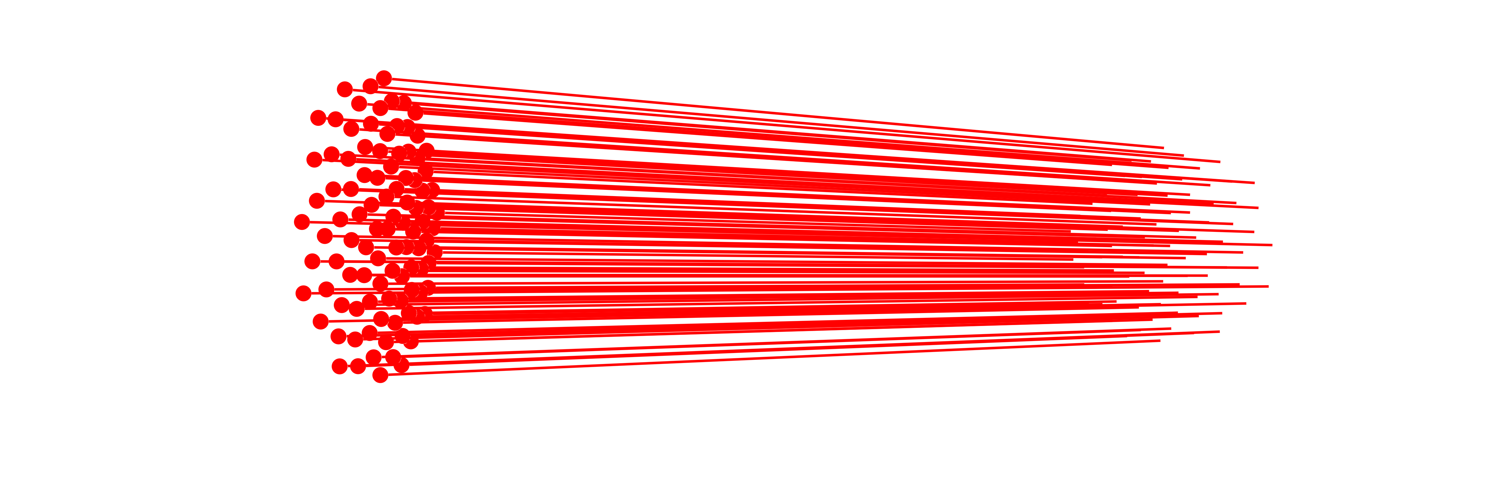
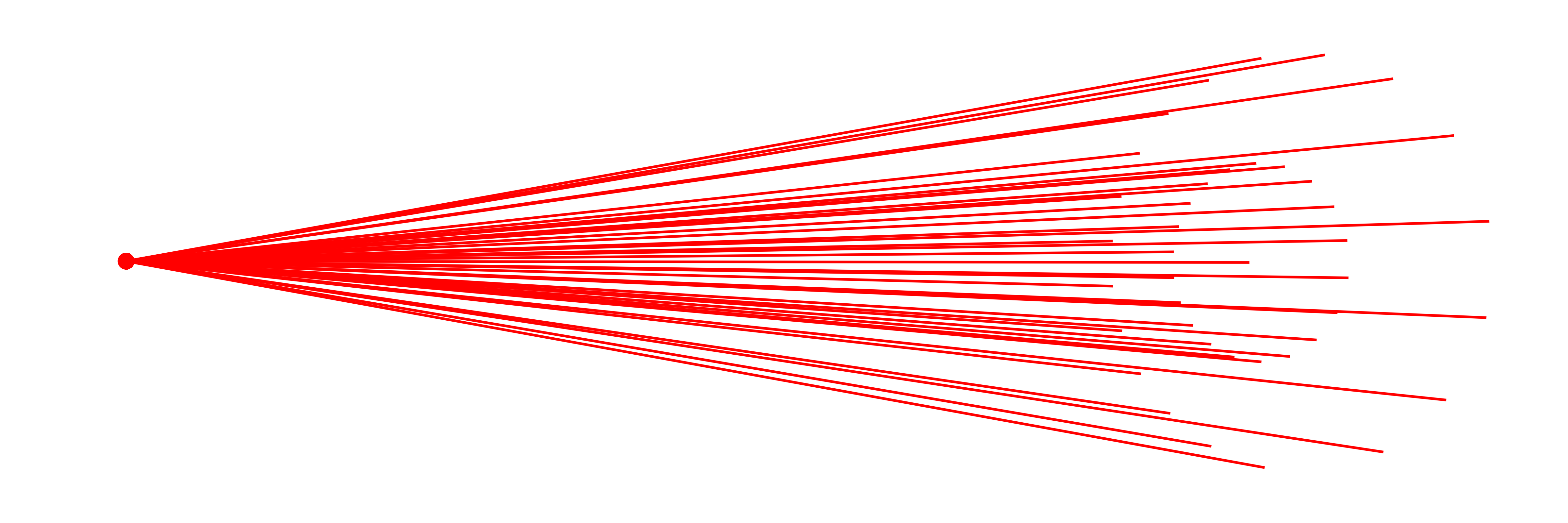
Below you can find an exemplary illustration of a PointSource.

Analogous to UniformDiscSource, a special constructor called UniformPointSource is available, which samples the spherical cap around dir with an equal solid angle per ray (Fibonacci/sunflower pattern), rather than in concentric rings. It returns a plain PointSource.

BeamletOptics.UniformPointSource Function

UniformPointSource(pos, dir, θ, λ; num_rays=1_000, basis)

Generates a cone of Beams emitted from pos with equal solid angle per ray across the spherical cap 0 ≤ ϑ ≤ θ around dir, using the deterministic sunflower (Fibonacci) pattern. The spiral starts with the center ray along dir (k = 0). The polar angle ϑₖ of the k-th ray (k = 1 … N-1) follows from cos ϑₖ = 1 - (k + ½)/N ⋅ (1 - cos θ), its azimuth is k times the golden angle π(3 - √5).

Note

This is merely a PointSource constructor which uses Fibonacci sampling instead of concentric rings. All rays are equally weighted samples of the cap: ray k represents the part of the cap with 1 - (k + 1)/N ⋅ (1 - cos θ) ≤ cos ϑ ≤ 1 - k/N ⋅ (1 - cos θ). The center ray represents the innermost of these parts, a cap, by its center.

Arguments

The following inputs and arguments can be used to configure the underlying PointSource:

Inputs

• pos: starting position of all beams

• dir: central source direction, i.e. the cone axis

• θ: half spread angle in rad, must be < π

• λ = 1e-6: wavelength in [m], default val. is 1000 nm

Keyword Arguments

• num_rays=1000: total number of rays in the source, must be ≥ 1

• basis: Optional reference vector (e.g. [1,0,0]) to define the starting azimuthal angle of the sunflower pattern. Must not be zero or parallel to dir.

Reproducible sampling

If no basis is passed, the orthogonal basis vectors are derived from dir deterministically, so two sources sharing the same dir, θ and num_rays sample exactly the same ray directions. Pass a basis to rotate the sunflower pattern about its own axis, e.g. to interleave several otherwise identical sources.

source

Line and fan sources

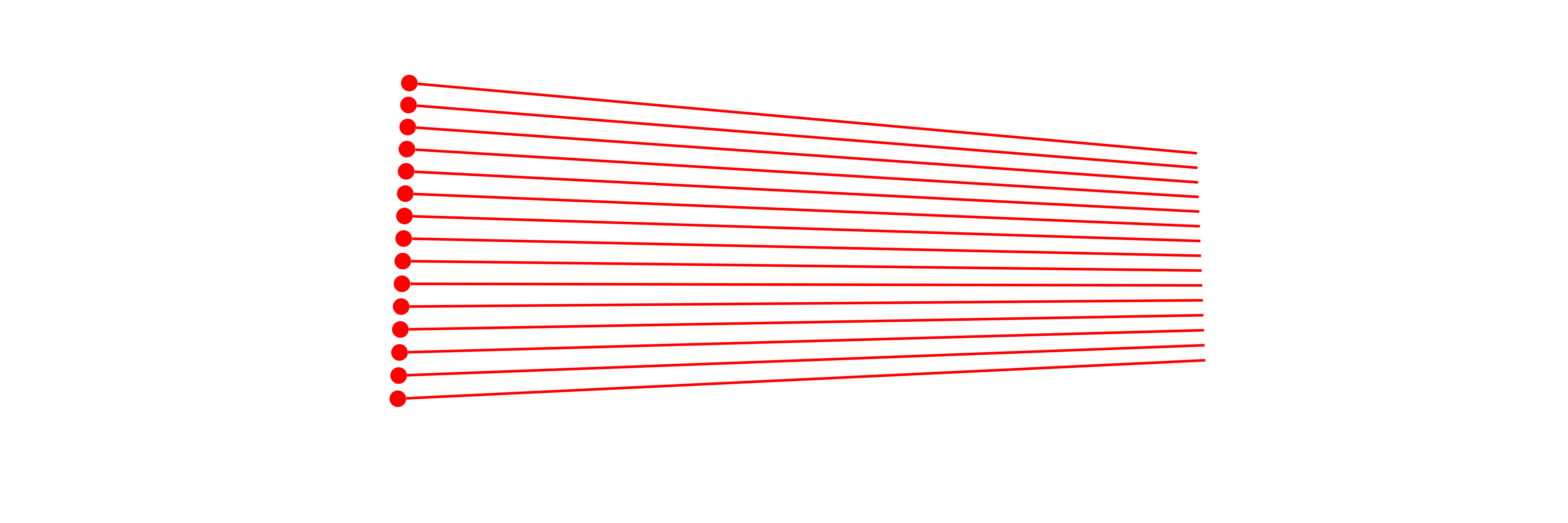
For layout sketches, or to trace only one section of a system (e.g. the meridional plane), a two-dimensional source is often sufficient. The UniformLineSource is the two-dimensional counterpart of the collimated source: a plane sheet of parallel Beams that start equidistantly on a line. It returns a plain CollimatedSource.

BeamletOptics.UniformLineSource Function

UniformLineSource(pos, dir, width, λ; num_rays=101, basis)

Generates a plane sheet of parallel Beams, i.e. a two-dimensional collimated source: the rays start equidistantly on a line of the length width centered at pos and travel along dir. The line lies along basis, such that all rays lie in the plane spanned by dir and basis. This is useful for layout sketches and for tracing a single (e.g. meridional or sagittal) section of a system.

The first ray is the center ray at pos. It is followed by h = (N - 1) ÷ 2 rays on each side of it, at pos + j/h ⋅ width/2 ⋅ basis for j = -h … h without j = 0, i.e. from one marginal ray at the end of the line to the other. A single ray starts at pos.

Use an odd number of rays

A pattern that is symmetric to its center ray has an odd number of rays. An even num_rays yields the pattern of num_rays - 1 rays and a second ray at pos.

Note

This is merely a CollimatedSource constructor which samples one diameter of the disc instead of concentric rings. width is stored as the diameter of the source.

Warning

The rays sample a line, not an area: they are not equal-area samples of a circular pupil. For a point spread function or an intensity use UniformDiscSource.

Arguments

The following inputs and arguments can be used to configure the underlying CollimatedSource:

Inputs

• pos: center of the line, i.e. the source position

• dir: starting direction of all beams

• width: length of the line in [m], i.e. the distance between the marginal rays

• λ = 1e-6: wavelength in [m]

Keyword Arguments

• num_rays=101: total number of rays in the source, must be ≥ 1

• basis: direction of the line (e.g. [1,0,0]), projected into the plane normal to dir. Must not be zero or parallel to dir.

Orientation of the line

If no basis is passed, the direction of the line is derived from dir deterministically via normal3d, which is rarely the section of interest: pass a basis to choose the plane of the rays. The line can also be turned about dir afterwards with rotate3d!.

source

The UniformFanSource is the two-dimensional counterpart of the point source: a plane fan of Beams from a single point with equidistant angles. It returns a plain PointSource.

BeamletOptics.UniformFanSource Function

UniformFanSource(pos, dir, θ, λ; num_rays=101, basis)

Generates a plane fan of Beams emitted from pos, i.e. a two-dimensional point source: the rays lie in the plane spanned by dir and basis, with equidistant angles between -θ and θ to dir. This is useful for layout sketches and for tracing a single (e.g. meridional or sagittal) section of a system.

The first ray is the center ray along dir. It is followed by h = (N - 1) ÷ 2 rays on each side of it, which enclose the angles φⱼ = j/h ⋅ θ with dir for j = -h … h without j = 0 and point along cos φⱼ ⋅ dir + sin φⱼ ⋅ basis, i.e. from one marginal ray at the edge of the fan to the other. A single ray points along dir.

Use an odd number of rays

A pattern that is symmetric to its center ray has an odd number of rays. An even num_rays yields the pattern of num_rays - 1 rays and a second ray along dir.

Note

This is merely a PointSource constructor which samples one section of the cone instead of concentric rings.

Warning

The rays sample a plane angle, not a solid angle: they are not equal solid angle samples of a cone. For a point spread function or an intensity use UniformPointSource.

Arguments

The following inputs and arguments can be used to configure the underlying PointSource:

Inputs

• pos: starting position of all beams

• dir: central source direction, i.e. the axis of the fan

• θ: half spread angle in rad, must be < π

• λ = 1e-6: wavelength in [m], default val. is 1000 nm

Keyword Arguments

• num_rays=101: total number of rays in the source, must be ≥ 1

• basis: direction (e.g. [1,0,0]) that spans the plane of the fan together with dir, projected into the plane normal to dir. Rays with a positive angle are tilted towards it. Must not be zero or parallel to dir.

Orientation of the fan

If no basis is passed, the plane of the fan is derived from dir deterministically via normal3d, which is rarely the section of interest: pass a basis to choose the plane of the rays. The fan can also be turned about dir afterwards with rotate3d!.

source

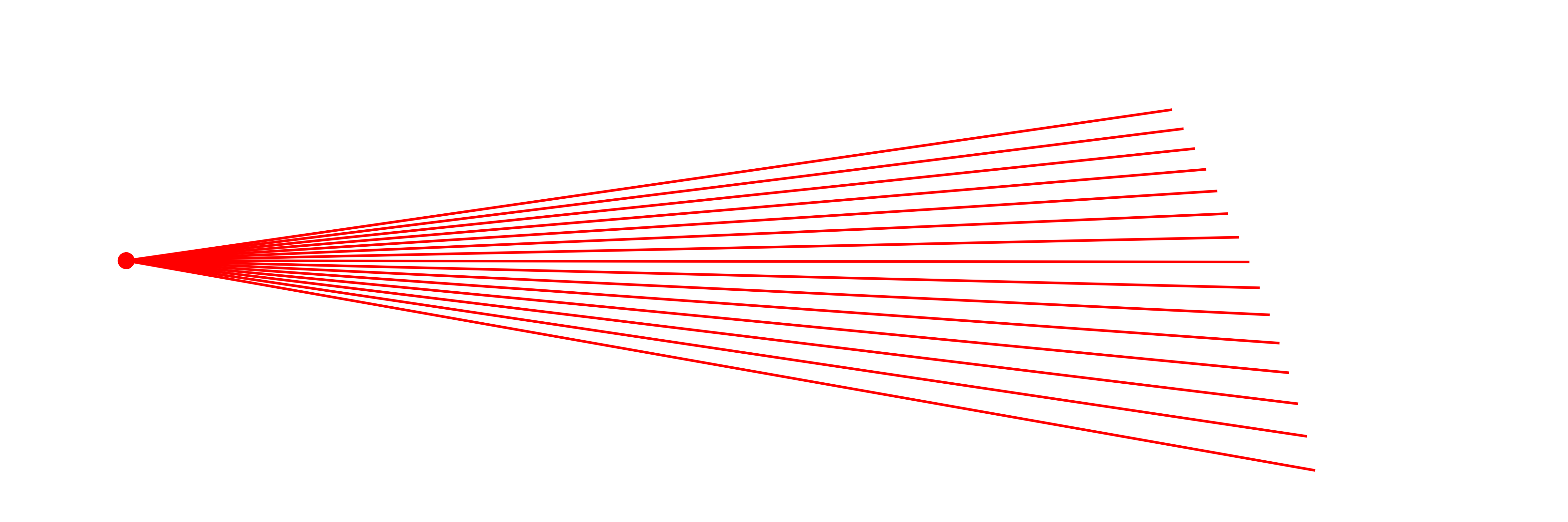
Both sources include the marginal rays and should be used with an odd number of rays. The plane of the rays is spanned by dir and the basis keyword argument. The rays stay in this plane only if the system is symmetric with respect to it. Since the rays sample a line or a plane angle instead of an area or a solid angle, these sources are not suited for calculating a point spread function with the intensity function.

Sampling and number of rays

A CollimatedSource or PointSource stores how its rays were sampled, such that num_rays! can regenerate them with another number of rays in the current pose of the source. How the beams are generated and how to add an own sampling is described in Source sampling.

The catalog constructors above build their sampling and call the generic constructors, which take the sampling as an argument:

BeamletOptics.CollimatedSource Method

CollimatedSource(pos, dir, diameter, sampling::AbstractSourceSampling, λ = 1e-6; num_rays, basis = nothing)

Spawns a CollimatedSource of parallel Beams along dir from a disc with the diameter [m] centered at pos [m], with the wavelength λ [m], sampled by sampling with num_rays rays, e.g. BeamletOptics.DiscRings. The catalog constructors CollimatedSource, UniformDiscSource and UniformLineSource call this method; a custom BeamletOptics.AbstractSourceSampling implements source_beams for it. The number type is promote_type of pos, dir, diameter and λ.

The optional basis vector sets the azimuth of the sampling pattern about dir, see BeamletOptics.sampling_basis. A num_rays below BeamletOptics.min_num_rays of the sampling and a basis that is zero or parallel to dir throw an ArgumentError.

source

BeamletOptics.PointSource Method

PointSource(pos, dir, sampling::AbstractSourceSampling, λ = 1e-6; num_rays, basis = nothing)

Spawns a PointSource of Beams emitted from pos [m] around the central direction dir with the wavelength λ [m], sampled by sampling with num_rays rays, e.g. BeamletOptics.ConeRings. The catalog constructors PointSource, UniformPointSource and UniformFanSource call this method; a custom BeamletOptics.AbstractSourceSampling implements source_beams and numerical_aperture for it. The number type is promote_type of pos, dir and λ.

The optional basis vector sets the azimuth of the sampling pattern about dir, see BeamletOptics.sampling_basis. A num_rays below BeamletOptics.min_num_rays of the sampling and a basis that is zero or parallel to dir throw an ArgumentError.

source

BeamletOptics.num_rays! Function

num_rays!(group, n)

Regenerates the rays of the source group with n rays: a CollimatedSource or PointSource, including UniformDiscSource, UniformPointSource, UniformLineSource and UniformFanSource. The rays are sampled as by the constructor of the source (concentric rings with the same num_rings, the sunflower pattern, or the line or fan), in the current pose of the source and at its wavelength, i.e. the source equals a new one with num_rays = n at its position and orientation. The rays start at the emission point of the current rays, also if set_pivot3d! moved the pivot of the source away from it. The previous beams, including their traced rays, are replaced: solve the system again afterwards. Returns group.

n must be at least BeamletOptics.min_num_rays of the source, i.e. 20 num_rings for ring sources and 1 for sunflower, line and fan sources, otherwise an ArgumentError is thrown, like by the constructors, and the source keeps its rays. A source built from given beams, e.g. CollimatedSource(beams, diameter, pos, dir), can not be regenerated and throws an ArgumentError.

source

Astigmatic Beam Groups

For complex sources, the package provides the AstigmaticBeamGroup container. Several constructors are available for different scenarios:

• GaussianBeamletDecomposition: Tiling a large Gaussian beam into many small stable beamlets.

• WavefrontBeamletDecomposition: Importing an arbitrary complex scalar field (e.g. from a phase screen or camera data), or a vector field with an independent, spatially varying polarization (e.g. OpticsBase's PlaneField, see OpticsBase fields as beam groups).

• CollimatedGaussianBeamletSource: A square grid of parallel beamlets (ideal for aperture diffraction).

• SphericalGaussianBeamletSource: A point-like source emitting a cone of beamlets (ideal for focused/divergent beams).

• EllipticalGaussianBeamletSource: A point-like source emitting an elliptical cone of beamlets (ideal for sources with different fast/slow axis divergence).

A field that is close to one Gaussian mode and too small to be tiled into beamlets, e.g. the output of a single-mode fiber, is not turned into a group: GaussianModeDecomposition fits a single AstigmaticGaussianBeamlet to it.

Existing beamlets are wrapped into a group with the constructor of the container:

BeamletOptics.AstigmaticBeamGroup Type

AstigmaticBeamGroup{T, R} <: AbstractBeamGroup{T, R}

A generic container for groups of AstigmaticGaussianBeamlets.

Fields

• beams: vector of all beamlets

• center: source position, pivot for rotations

• dir: the orientation of the group, a right-handed orthonormal matrix whose columns are the sampling reference vector, the central source direction and their cross product, see AbstractBeamGroup

source

BeamletOptics.AstigmaticBeamGroup Method

AstigmaticBeamGroup(beams, pos, dir::AbstractVector)
AstigmaticBeamGroup(beams, pos, orientation::AbstractMatrix)

Wraps existing beams into an AstigmaticBeamGroup with the source position pos. The group orientation is either derived from the central direction dir (the sampling reference vector is then picked deterministically via normal3d), or passed explicitly as a right-handed orthonormal 3x3 orientation matrix whose second column is the central direction. An invalid orientation throws an ArgumentError.

source

The beamlet sources and the decomposition of a Gaussian beam are generated by

BeamletOptics.CollimatedGaussianBeamletSource Method

CollimatedGaussianBeamletSource(pos, dir, D, λ, w0s; n_grid=20, P0)

Generates an n_grid × n_grid square array of AstigmaticGaussianBeamlets, all pointing in the same direction and having the same uniform amplitude. This is used to model macroscopic plane waves or flat-top beams passing through hard apertures (e.g., for Fraunhofer or Fresnel diffraction).

Arguments

• pos: Center position of the source plane.

• dir: Propagation direction.

• D: Total width/height of the square aperture.

• λ: Wavelength.

• w0s: Sub-waist of each individual beamlet. For smooth overlap, w0s ≈ D / n_grid.

• n_grid: Number of beamlets along one axis (default 20 yields 400 total beamlets).

• basis: Optional tuple (ex, ey) of the macroscopic sampling grid axes, i.e. the 3D directions corresponding to the x and y grid axes. ex must not be zero or parallel to dir; its component normal to dir becomes the local x-axis of the group orientation.

• randomize_axes: If true, the internal principal axes of each individual beamlet are randomly rotated. This averages out numerical grid-alignment biases and is essential for preserving rotational symmetry in focused spots (e.g. Airy disks).

• rng: Random number generator to use for randomize_axes.

• P0: Total power of the source in [W]. The beamlets overlap and add coherently; their fields are scaled such that the superposition carries P0.

source

BeamletOptics.SphericalGaussianBeamletSource Method

SphericalGaussianBeamletSource(pos, dir, θ, λ; num_rings=10, num_rays=100*num_rings)

Decomposes a macroscopic spherical wave (or a highly divergent/focused beam) into a cone of AstigmaticGaussianBeamlets originating from a single point pos.

The angular spread of the beamlets is bounded by the half-angle θ. To ensure a smooth far-field interference pattern without speckle, the sub-waist w0s of each beamlet is automatically calculated such that their far-field divergence perfectly overlaps with adjacent beamlets in the grid.

Arguments

• pos: Origin point of the spherical wave.

• dir: Central propagation direction.

• θ: Half spread angle in radians.

• λ: Wavelength.

• num_rings: Number of concentric angular rings; the number of rings counts the center as the innermost one, i.e. num_rings - 1 rings lie around it.

• num_rays: Total number of beamlets to generate.

• overlap: Scaling factor for the sub-waist divergence (default 1.2 ensures smooth overlap).

• basis: Optional reference vector (e.g. [1,0,0]) to define the starting azimuthal angle for the source rings.

• randomize_axes: If true, the internal principal axes of each individual beamlet are randomly rotated. This averages out numerical artifacts in the far-field focus.

• rng: Random number generator to use for randomize_axes.

• P0: Total power of the spherical source in [W]. The beamlets overlap and add coherently in the far field; their fields are scaled such that the superposition carries P0.

• E0: Optional Jones vector defining the polarization and phase of the spherical wave; its component transverse to each beamlet is used, its magnitude does not matter, the power is P0.

Reproducible sampling

If no basis is passed, the orthogonal basis vectors are derived from dir deterministically, so two sources sharing the same arguments sample exactly the same beamlet directions. Pass a basis to rotate the azimuthal sampling of a source about its own axis. A basis that is zero or parallel to dir throws.

source

BeamletOptics.EllipticalGaussianBeamletSource Method

EllipticalGaussianBeamletSource(pos, dir, θ_x, θ_y, λ; num_rings=10, num_rays=100*num_rings, ...)

Spawns a coherent array of AstigmaticGaussianBeamlets distributed on an elliptical cap. This is ideal for modelling sources with different divergences in the fast and slow axes, such as tapered amplifiers or edge-emitting laser diodes.

Arguments

• pos: Origin point of the spherical wave.

• dir: Central propagation direction.

• θ_x, θ_y: Half spread angles in radians for the two principal axes.

• λ: Wavelength.

• num_rings: Number of concentric angular rings; the number of rings counts the center as the innermost one, i.e. num_rings - 1 rings lie around it.

• num_rays: Total number of beamlets to generate.

• overlap: Scaling factor for the sub-waist divergence (default 1.2 ensures smooth overlap).

• basis: Optional reference vector (e.g. [1,0,0]) to define the starting azimuthal angle for the source rings.

• randomize_axes: If true, the internal principal axes of each individual beamlet are randomly rotated.

• rng: Random number generator to use for randomize_axes.

• P0: Total power of the source in [W]. The beamlets overlap and add coherently in the far field; their fields are scaled such that the superposition carries P0.

• E0: Optional Jones vector defining the polarization and phase of the wave; its component transverse to each beamlet is used, its magnitude does not matter, the power is P0.

Reproducible sampling

If no basis is passed, the orthogonal basis vectors are derived from dir deterministically, so two sources sharing the same arguments sample exactly the same beamlet directions. Pass a basis to rotate the azimuthal sampling of a source about its own axis. A basis that is zero or parallel to dir throws.

source

BeamletOptics.GaussianBeamletDecomposition Method

GaussianBeamletDecomposition(pos, dir, λ, w0; n_grid=20)

Decomposes a macroscopic Gaussian beam of waist w0 into an n_grid × n_grid array of microscopic AstigmaticGaussianBeamlets. This allows the accurate tracing of large Gaussian beams through highly aberrative or non-paraxial optical systems, perfectly preserving higher-order phase aberrations via the coherent superposition of the sub-beamlets.

Arguments

• pos: Waist center position of the macroscopic beam.

• dir: Propagation direction.

• λ: Wavelength.

• w0: Macroscopic beam waist.

• n_grid: Number of beamlets along one axis (default 20 yields 400 total beamlets). The grid spans 4 w0; the sub-waist overlap ⋅ 4 w0 / n_grid of the beamlets must be smaller than w0, i.e. n_grid > 4 overlap, else an ArgumentError is thrown. The superposition of the beamlets is the Gaussian beam of the waist w0 and the power P0: the sampled envelope is deconvolved with the profile of a beamlet.

• overlap: Scaling factor for the sub-waist relative to grid spacing (default 1.2 ensures smooth overlap).

• basis: Optional tuple (ex, ey) of the macroscopic sampling grid axes, i.e. the 3D directions corresponding to the x and y grid axes. ex must not be zero or parallel to dir; its component normal to dir becomes the local x-axis of the group orientation.

• randomize_axes: If true, the internal principal axes of each individual beamlet are randomly rotated. This averages out numerical grid-alignment biases and is essential for preserving rotational symmetry in focused spots.

• rng: Random number generator to use for randomize_axes.

• P0: Total power of the macroscopic Gaussian beam in [W].

• E0: Optional Jones vector defining the polarization and initial phase of the beam; its component transverse to dir is used, its magnitude does not matter, the power is P0. If nothing, defaults to linear polarization along the first grid axis.

• threshold: Relative amplitude below which beamlets are not spawned (default 1e-4).

source

and the decompositions of a sampled field, given as arrays, by

BeamletOptics.WavefrontBeamletDecomposition Method

WavefrontBeamletDecomposition(x, y, amplitude, phase, pos, dir, λ; threshold=1e-4)

Decomposes an arbitrary complex scalar field (defined by a spatial amplitude and phase distribution on a 2D grid x and y) into a collection of AstigmaticGaussianBeamlets.

This function uses the Eikonal approximation to map the local phase gradient into a local propagation direction for each beamlet. It allows users to import arbitrary, aberrated, or custom beam profiles (e.g. from a camera or a wavefront sensor) and propagate them through a BeamletOptics system.

The grid lies in the plane normal to dir through pos, the position of the sample x = y = 0 and the center of the group.

Arguments

• x, y: Vectors defining the 1D spatial coordinates of the 2D field grid, relative to pos.

• amplitude: 2D array of field amplitudes (length(x) × length(y)).

• phase: 2D array of phase values in radians.

• pos: global position of the sample x = y = 0 in [m].

• dir: The macroscopic reference propagation direction (e.g., [0, 1, 0]).

• λ: Wavelength.

• threshold: Relative amplitude threshold below which beamlets are not spawned (saves computation).

• overlap: Scaling factor for the sub-waist relative to grid spacing (default 1.2 ensures smooth overlap).

• basis: Optional tuple (ex, ey) of the macroscopic sampling grid axes, i.e. the 3D directions corresponding to the x and y input axes. ex must not be zero or parallel to dir; its component normal to dir becomes the local x-axis of the group orientation.

• randomize_axes: If true, the internal principal axes of each individual beamlet are randomly rotated. This averages out numerical grid-alignment biases and helps preserve rotational symmetry in focused patterns.

• rng: Random number generator to use for randomize_axes.

• E0: Optional reference polarization vector or Jones vector. If nothing, defaults to linear polarization along the first grid axis.

Sampling

The phase step between neighboring samples must stay below π: a field tilted by θ against dir needs dx < λ / (2 sin θ), while the beamlets (waist overlap * dx) must stay much larger than λ. Keep the sampling plane close to normal to the beam.

source

BeamletOptics.WavefrontBeamletDecomposition Method

WavefrontBeamletDecomposition(x, y, Eu, Ev, pos, dir, λ; threshold=1e-4)

Vector-field counterpart of WavefrontBeamletDecomposition(x, y, amplitude, phase, pos, dir, λ): decomposes a transverse complex vector field, given as its two components Eu, Ev along the sampling axes e1, e2 (basis, default e1 = normal3d(dir), e2 = dir × e1), into a collection of AstigmaticGaussianBeamlets.

Unlike the scalar method (one amplitude/phase pair plus a single macroscopic polarization E0), this method carries an independent complex amplitude per polarization component and grid point, i.e. an arbitrary, spatially varying polarization state (including elliptical and depolarizing-looking patterns coming from separate Eu, Ev measurements).

Arguments

• x, y: 1D spatial coordinates of the field grid, along e1, e2, relative to pos, in [m].

• Eu, Ev: length(x) × length(y) complex matrices, the field components along e1, e2 in [V/m] (peak amplitude). Both must have the full spatial phase.

• pos: global position of the sample x = y = 0 in [m], the center of the group.

• dir: macroscopic reference propagation direction (e.g. [0, 1, 0]).

• λ: wavelength in [m].

• threshold: relative amplitude (of hypot.(abs.(Eu), abs.(Ev))) below which no beamlet is spawned.

• overlap, basis, randomize_axes, rng: as in the scalar method.

• R: radius in [m] of a reference sphere that has been removed from Eu, Ev: the physical field is E .* cis(sign(R) k (√(x² + y² + R²) − |R|)) with k = 2π/λ (R > 0: diverging from the point at the distance R behind x = y = 0, R < 0: converging to the point |R| in front of it). Default Inf: Eu, Ev are the physical field. The sphere enters analytically, so the grid only has to resolve the phase of Eu, Ev, not that of the sphere: every beamlet travels along the ray of the sphere through its sample (plus the gradient of the sampled phase) and starts with the wavefront curvature of the sphere.

Throws an ArgumentError for a field that is zero everywhere and for R = 0.

Sampling

The phase step between neighboring samples must stay below π: a field tilted by θ against dir needs dx < λ / (2 sin θ), while the beamlets (waist overlap * dx) must stay much larger than λ. Keep the sampling plane close to normal to the beam. Both components must share one local wavevector at each sample.

source

BeamletOptics.GaussianModeDecomposition Method

GaussianModeDecomposition(x, y, Eu, Ev, pos, dir, λ; basis = nothing, R = Inf)

Fits a single AstigmaticGaussianBeamlet to a transverse complex vector field, given by its components Eu, Ev along the sampling axes e1, e2 of a plane normal to dir. This is the lowest-order Gaussian mode decomposition: the counterpart of WavefrontBeamletDecomposition for fields that are close to one Gaussian mode and too small to be tiled into many beamlets, e.g. the output of a single-mode fiber (beamlets must be much larger than λ).

Arguments

• x, y: 1D sample coordinates along e1, e2 in [m], relative to pos.

• Eu, Ev: length(x) × length(y) complex field components along e1, e2 in [V/m] (peak amplitude), with the full spatial phase and travelling along dir.

• pos: global position of the sample x = y = 0 in [m].

• dir: propagation direction, the normal of the sampling plane.

• λ: vacuum wavelength in [m]. The plane must lie in vacuum or air (n = 1), where BMO starts beams.

• basis: optional tuple (ex, ey) of the sampling axes e1, e2, as in WavefrontBeamletDecomposition. Default: e1 = normal3d(dir), e2 = dir × e1.

• R: radius in [m] of a reference sphere that has been removed from Eu, Ev, as in WavefrontBeamletDecomposition(x, y, Eu, Ev, pos, dir, λ). Default Inf: Eu, Ev are the physical field. The sphere enters the fit analytically (tilt at the centroid, curvature 1/R), so the grid only has to resolve the phase of Eu, Ev.

The beamlet starts at the centroid on the plane, with waist radii and waist positions along its principal axes that reproduce the fitted radii and curvatures there.

The beamlet carries only the projected part of the field: optical_power(beamlet) divided by the power of the input is the fraction of the power in the fitted Gaussian mode, i.e. the quality of the approximation.

Limits

The widths are measured in the plane, so the tilt of the fitted direction against dir must be small. A twist between the axes of curvature and intensity (general astigmatism) is not represented.

source

The decompositions of a sampled field take the grid position as a positional argument, like every other source: WavefrontBeamletDecomposition(x, y, amplitude, phase, pos, dir, λ), WavefrontBeamletDecomposition(x, y, Eu, Ev, pos, dir, λ) and GaussianModeDecomposition(x, y, Eu, Ev, pos, dir, λ). The grid lies in the plane normal to dir through pos, and pos is the global position of the sample x = y = 0. For the two WavefrontBeamletDecomposition forms, pos is also the center of the returned group; the single beamlet of GaussianModeDecomposition starts at the centroid of the field on that plane.

Beamlet sources and decompositions

The beamlet sources and decompositions normalize the beamlets such that their coherent superposition is the intended field. This section collects how.

Gaussian beamlet decomposition. The superposition of the beamlets of GaussianBeamletDecomposition is the sampled envelope convolved with a beamlet. For a Gaussian envelope of the waist it is a Gaussian of the waist and the peak amplitude  , with the sub-waist of the beamlets. The envelope is therefore deconvolved, such that the superposition is the macroscopic beam of the waist w0, its peak amplitude and its power P0.

Power of a tilted beamlet. In WavefrontBeamletDecomposition, each beamlet represents a cell of the area . The footprint of a beamlet tilted by against dir is stretched by on the sampling plane, so the Gaussian overlap integral there is , and the field is scaled by .

Local propagation direction and polarization of the vector field. In the vector-field method of WavefrontBeamletDecomposition, the local propagation direction at each grid point is found from the Eikonal equation, with the phase difference between neighboring samples taken from the complex vector overlap . This is continuous where the polarization changes and assumes that both components share one local wavevector, i.e. that the field is not the superposition of two waves with genuinely different directions at that point. The phase step between neighbors must stay below : a field tilted by against dir needs  , while the beamlets (waist overlap * dx) must stay much larger than , so keep the sampling plane close to normal to the beam.

The E0 of a beamlet keeps the given tangential components Eu, Ev and gets the normal component that makes it transverse to the local direction (  ). Its amplitude is scaled by   , because the footprint of a tilted beamlet on the sampling plane is stretched by . The sum of the beamlets then reproduces the sampled tangential field for oblique beams as well.

Fit of the Gaussian mode decomposition. GaussianModeDecomposition fits its beamlet in five steps:

1. Polarization: the dominant eigenvector of the coherence matrix ; the field is projected onto it.

2. Position and waist: centroid and principal axes of the second intensity moments; the beam radius along a principal axis is twice the rms width.

3. Direction: the mean transverse wave vector, from the intensity-weighted phase step between neighboring samples.

4. Curvature: the quadratic phase from the moments of the phase gradient (phase steps between neighbors), taken along the principal axes of the intensity. Twist between curvature and intensity axes (general astigmatism) is not represented.

5. Amplitude and phase: the projection of the field onto the fitted mode.

Coherent power of beamlet sources. CollimatedGaussianBeamletSource, SphericalGaussianBeamletSource and EllipticalGaussianBeamletSource emit beamlets of equal power that start in phase. Their profiles are Gaussians of the width (the half width of the intensity) about vectors in a common plane: the positions with the waist in the source plane of collimated beamlets, or the directions with the far-field divergence of beamlets from one point. Where the beamlets overlap, their fields add: two beamlets of the power whose vectors differ by contribute   to the power of the superposition per pair, i.e. it carries with     instead of (pairs farther apart than are left out of the sum). The fields of all beamlets are multiplied by the same factor , such that the superposition carries the sum of their powers. The factor does not depend on the beamlet, so beamlets at the edge of the source, where fewer neighbors overlap, are scaled like those in the center.

OpticsBase fields as beam groups

With using OpticsBase, a PlaneField handed over by another solver (e.g. the exit field of a fiber computed by a beam propagation method) becomes BMO beams again. WavefrontBeamletDecomposition tiles it into one beamlet per sample, which needs beamlets much larger than λ. GaussianModeDecomposition fits a single Gaussian beamlet instead, for small fields close to one Gaussian mode such as single-mode fiber output. Both take only the forward-travelling part of the field and require the plane to lie in vacuum or air. The detector side, PlaneField(::Detector), is described under OpticsBase interoperability.

Details of the PlaneField return path:

• The field used is forward(f).E .* reference_phase(f) in [V/m] peak amplitude, matching the units AstigmaticGaussianBeamlet's E0 expects. forward(f) is the stored array with the local-plane-wave forward/backward split applied, and reference_phase(f) the phase of the reference sphere (if any). The samples and the sphere are handed on separately (R = f.R), so the grid only has to resolve the phase of the stored array, not that of the sphere. For GaussianModeDecomposition the sphere likewise enters the fit analytically.

• Only the forward part is decomposed, because a PlaneField has no ready single propagation direction for its backward part, while the constructor needs one direction per call. A field without forward light (e.g. a purely backward wave, whose forward part is rounding noise) cannot be decomposed.

• forward splits each sample as a local plane wave along the reference direction. A beam at the angle to it loses an amplitude of the order  . Keep the plane close to normal to the beam, which the beamlet size requires anyway (see WavefrontBeamletDecomposition).

• f must lie in vacuum or air (f.n == 1): BMO starts beams in vacuum, and a field in a medium would need a medium-to-vacuum conversion of amplitude and optical path. An ArgumentError is thrown otherwise.

• Passing the result of PlaneField(detector; ...) back into WavefrontBeamletDecomposition and tracing the resulting beam group reproduces the original field (round trip), up to beamlet-grid discretization error.

BeamletOptics.WavefrontBeamletDecomposition Method

BeamletOptics.WavefrontBeamletDecomposition(f::OpticsBase.PlaneField; kwargs...)

Decomposes the forward-travelling part of a PlaneField f into an AstigmaticBeamGroup of AstigmaticGaussianBeamlets, placed on f's plane and travelling along f's normal n. This is the return path for OpticsBase.PlaneField(detector; ...).

Arguments

• f: the field to decompose. Only forward(f) (the part travelling along +n) is used; the backward part is dropped.

• kwargs...: forwarded to WavefrontBeamletDecomposition(x, y, Eu, Ev, pos, dir, λ; kwargs...) (threshold, overlap, randomize_axes, rng); basis is fixed to f's own (u, v) and R to f.R, neither can be overridden.

Conventions

• The physical field used is forward(f).E .* reference_phase(f), in [V/m] peak amplitude, matching the units AstigmaticGaussianBeamlet's E0 expects. The samples and the reference sphere are handed on separately (R = f.R).

• The beam group is placed at f.origin (pos = f.origin) with the local axes f.axes[:, 1:2]; its sampling grid is f's own (u, v) grid (OpticsBase.coordinates).

• f must lie in vacuum or air (f.n == 1).

Warning

forward splits each sample as a local plane wave along the reference direction (n for R = Inf); a beam at the angle θ to it loses an amplitude of the order (1 − cos θ)/2. Keep the plane close to normal to the beam.

Throws an ArgumentError if f.n != 1, if f has no forward-travelling light (e.g. a purely backward wave), or if kwargs contains basis or R, and whatever WavefrontBeamletDecomposition(x, y, Eu, Ev, pos, dir, λ) throws.

source

BeamletOptics.GaussianModeDecomposition Method

BeamletOptics.GaussianModeDecomposition(f::OpticsBase.PlaneField)

Fits a single AstigmaticGaussianBeamlet to the forward-travelling part of a PlaneField, e.g. the output of a single-mode fiber. The beamlet starts on f's plane at the centroid of the field; see GaussianModeDecomposition for the fit. Use it for fields close to one Gaussian mode that are too small for WavefrontBeamletDecomposition (which needs beamlets much larger than λ).

optical_power(beamlet) / OpticsBase.power(f) is the fraction of the power captured by the Gaussian mode. The field used is forward(f).E .* reference_phase(f), with the reference sphere passed on as R = f.R. f must lie in vacuum or air (f.n == 1) and must contain forward-travelling light; an ArgumentError is thrown otherwise.

source