Astigmatic polarized beamlets

Standard stigmatic beamlets are limited to symmetric systems. For the modeling of arbitrary optical systems, including off-axis components, tilted lenses, or complex media like atmospheric turbulence, the package provides the AstigmaticGaussianBeamlet. This type implements the astigmatic Gaussian beamlet ray tracing formalism initially proposed by Greynolds (1986) [15, 16].

However, this idea has been referred to in multiple ways over the last few decades, including but not limited to: Gaussian Beamlet Tracing (GBT), Fat Ray Tracing (FRT), Parabasal Ray Tracing (PRT), Complex Ray Tracing (CRT), Gauss Beamlet Propagation (GBP) and Beam Synthesis Propagation (BSP).

Formalism

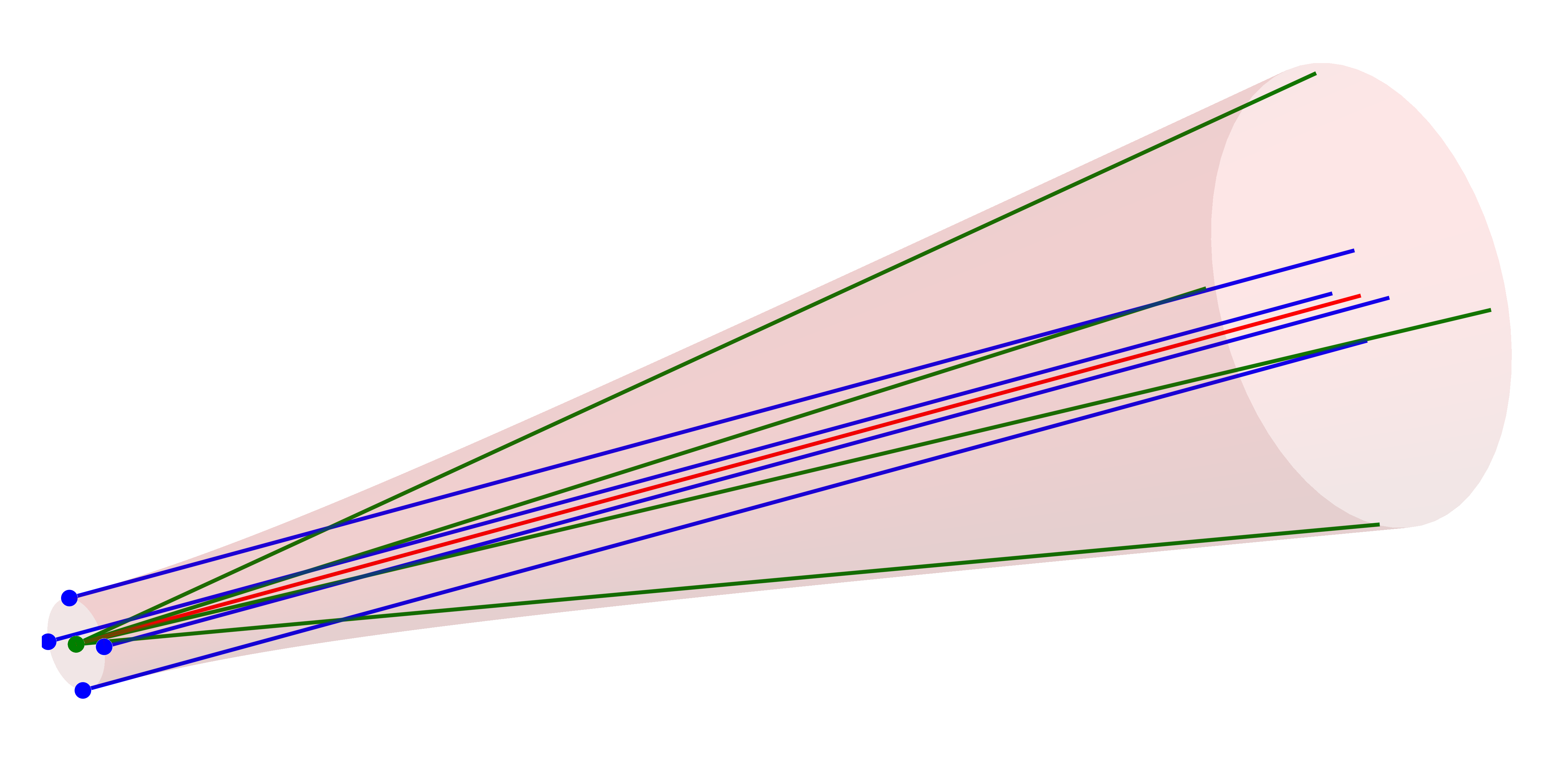
Similar to the Gauss model presented in the Stigmatic beamlets chapter, an astigmatic beamlet can represented by a cluster of 9 rays:

Ray representation

1. Chief Ray: a PolarizedRay defining the central path and polarization state.

2. Waist Rays: four "positional" rays (waist     )

3. Divergence Rays: four "directional" rays (divergence     )

These rays can be thought of tracking the complex curvature matrix through the system. The key assumptions made in order for this formalism to hold are:

Key assumptions

1. Paraxiality: the auxiliary rays must remain within the paraxial regime relative to the chief ray.

2. Parabolic interaction: since only astigmatism can be captured, each surface interaction must be approximately parabolical

3. Homogeneous polarization: the polarization state of the traced field is assumed to be homogeneous over each beamlet

4. Matched scale: the beamlet must be smaller than the optical element it interacts with, see also 2.

The initial ordering of the geometric beams/rays is shown in the figure below. The colors represent the chief (red), waist (blue) and divergence (green) beams.

As with the GaussianBeamlet, tracing these rays through a system allows the reconstruction of the waist envelope and electric field. The reduced complex amplitude of the Gaussian beamlet is computed as

where and are the two-dimensional complex ray height and angle vectors on the plane perpendicular to the chief ray [15, 17, 18]. The second exponential is the Gaussian envelope   with the spot matrix , and   , see Physical Beam Cross-Section. By also tracing a 3D-field vector along the chief ray based on the formalism introduced in the Polarized rays section, polarization effects can be considered when calculating [19]. For a simple lens setup, the resulting waist is illustrated in the image below.

The linear polarization state is visualized by an oscillating red line and is proportional to the on-axis peak field strength.

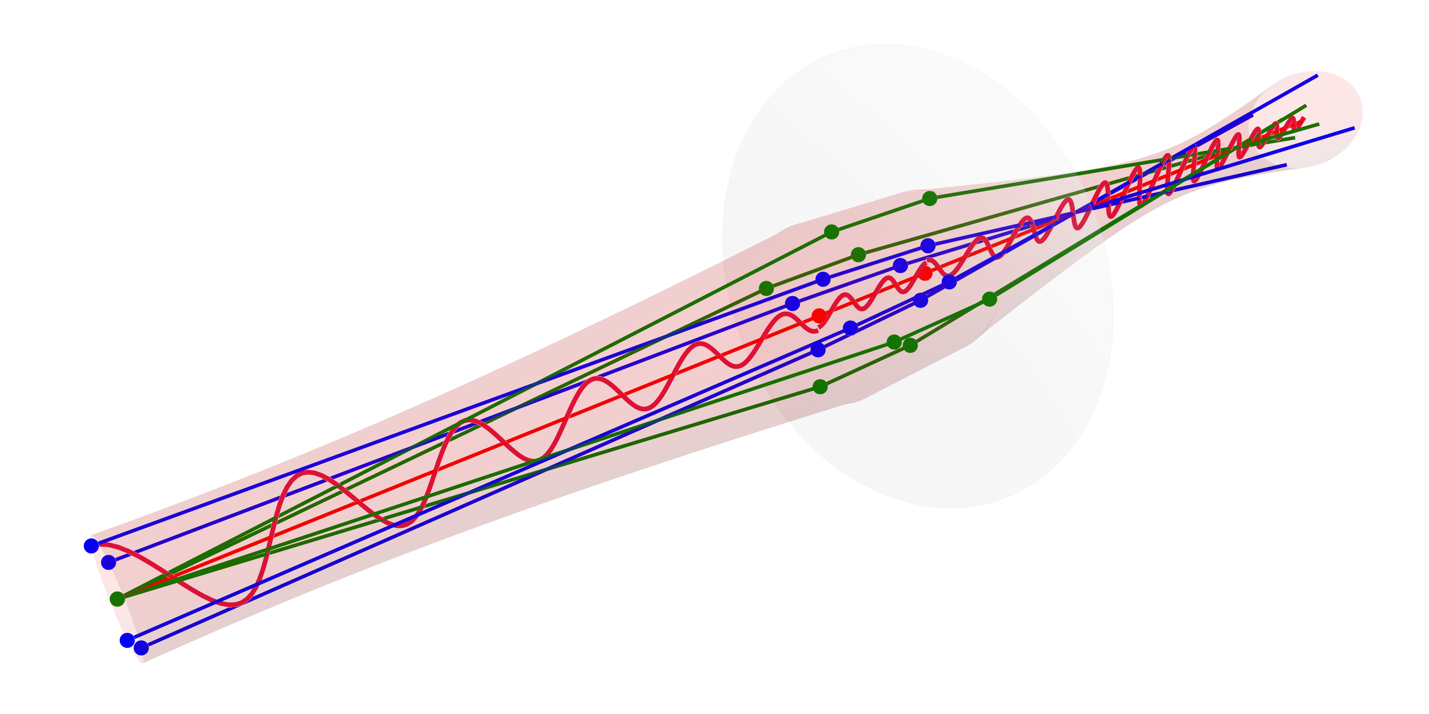
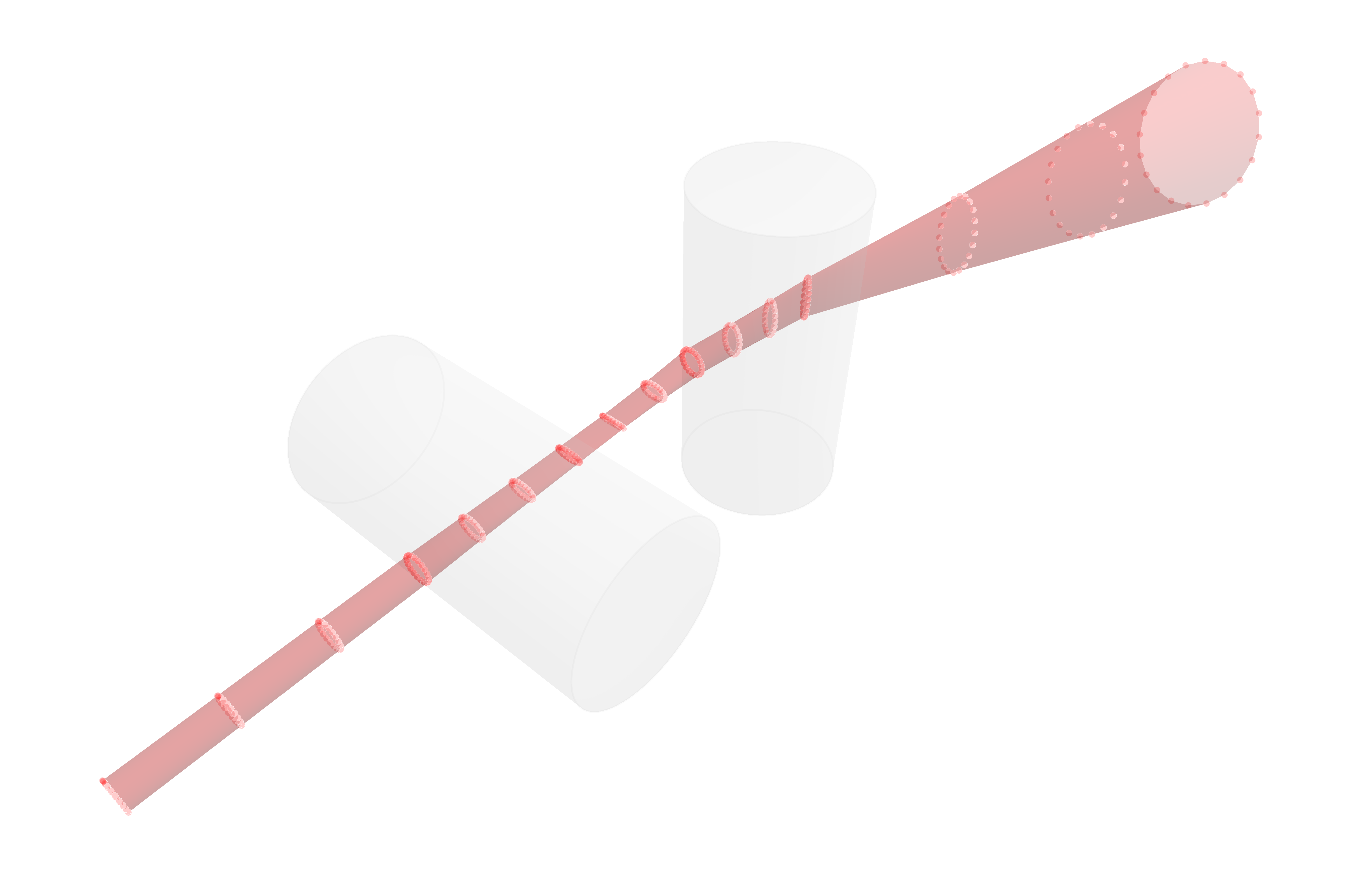
While the above beam closely matches the example Gaussian given in the previous section (Obtaining the beam parameters), the real advantage of this extended method lies in the tracing of non-symmetric systems. For a tilted two cylinder lens system, the following result with strong astigmatic effects is obtained. Multiple waist slices are marked with red dots.

The phase factor due to the optical path length of the central ray () is added to the reduced field during the final field calculation for each beamlet. More information on the mathemathics behind this formalism can be found below in The Curvature Matrix section.

Optical invariant

In order to ensure the correctness of the traced beamlet, the complex ray vectors must satisfy the vanishing complex optical invariant:

with the analytic bilinear form of the dot product (see below). Tracing stops with a warning if its absolute value exceeds get_invariant_threshold(), by default . This ensures that the complex curvature matrix is symmetric, since the beamlet formalism can not capture higher-order abberations.

The Lagrange invariant    of each axis must keep its value at the start of the beam, . A large beamlet in a strong focus does not: the rays leave the parabolic part of the surface and of one axis can even change its sign, as happens for separate waists. Tracing stops with a warning if deviates by more than get_lagrange_tolerance(), by default 50 %, from its start value, for any and wavelength.

Astigmatic beamlets

You can construct a single astigmatic beamlet with a specified waist and polarization:

BeamletOptics.AstigmaticGaussianBeamlet Method

AstigmaticGaussianBeamlet(position, direction, λ, w0; kwargs...)

Constructs an astigmatic Gaussian beamlet at position with the specified beam parameters. In the 4-argument version, the beam has circular symmetry with waist radius w0. In the 5-argument version, independent waists w0_x and w0_y can be specified.

Arguments

Inputs

• position: origin of the beamlet

• direction: direction of the beamlet

• λ: wavelength of the beamlet in [m]. Default value is 1000 nm.

• w0: beam waist (radius) in [m]. Default value is 1 mm.

• w0_x, w0_y: independent beam waists in [m].

Keyword Arguments

• M2, M2_x, M2_y: beam quality factors. Default is 1

• P0: beam total power in [W]. Default is 1 mW.

• E0: electric field vector in [V/m] at position, it replaces P0. Default is nothing (aligned with support axes, scaled by P0, zero Gouy phase at the waist).

• support: optional support vector for basis construction, i.e. the X axis of the beamlet. Must be orthogonal to direction, otherwise an ArgumentError is thrown; has any non-zero length and is normalized internally. Default is nothing, i.e. a vector orthogonal to direction is chosen.

• z0: beam waist offset in [m]. Default is 0 m

Additional information

Waist offset

As for a GaussianBeamlet, the z0 keyword arg. spawns a beam at the specified position with its waist at an offset z0 in [m] along the chief ray axis.

Optical invariant check

When using the solve_system! function, the beamlet invariant will be checked for each interaction. If the invariant is violated, tracing will be stopped.

source

Independent waists in the two transverse axes, e.g. of a diode laser, are set with the five-argument constructor:

BeamletOptics.AstigmaticGaussianBeamlet Method

AstigmaticGaussianBeamlet(position, direction, λ, w0_x, w0_y; kwargs...)

Constructs an astigmatic Gaussian beamlet with independent waists w0_x and w0_y. This constructor supports modeling astigmatic sources where the waists in X and Y are at different locations along the beam axis.

Arguments

• position: Origin of the beamlet.

• direction: Propagation direction vector.

• λ: Wavelength.

• w0_x: Waist radius in the X direction (defined by the support vector).

• w0_y: Waist radius in the Y direction.

Keyword Arguments

• z0_x: Offset of the X waist from position along the propagation axis in [m]. Defaults to z0.

• z0_y: Offset of the Y waist from position along the propagation axis in [m]. Defaults to z0.

• z0: Default for z0_x and z0_y. Default is 0 m.

• M2_x, M2_y: Beam quality factors. Default is 1.

• P0: Total power in [W].

• E0: Optional electric field vector in [V/m] at position, it replaces P0.

• support: Optional vector orthogonal to direction to define the X axis. Has any non-zero length and is normalized internally. A support that is not orthogonal to the direction (the dot product of the unit vectors exceeds get_orthogonality_threshold(), default 1e-10) throws an ArgumentError. Default is nothing, i.e. a vector orthogonal to direction is chosen.

Additional information

Optical invariant check

When using the solve_system! function, the beamlet invariant will be checked for each interaction. If the invariant is violated, tracing will be stopped.

source

The constructor will spawn an AstigmaticGaussianBeamlet which is implemented as follows:

BeamletOptics.AstigmaticGaussianBeamlet Type

AstigmaticGaussianBeamlet{T} <: AbstractBeam{T, PolarizedRay{T}}

Complex ray representation of a general astigmatic Gaussian beam as per the formalism described by A. Greynolds (1986) and N. Worku (2017). The beam is described by a chief PolarizedRay and 8 auxiliary Rays that encode the waist radius and divergence in two orthogonal transverse axes. The beam quality M2 is considered via the divergence angle. All equations are based on the following publications:

Alan Greynolds, "Vector formulation of the ray-equivalent method for general Gaussian beam propagation." Curr. Dev. Opt. Eng. Diffraction Phenom. Vol. 679. SPIE, 1986

and

Norman Worku and Herbert Gross, "Vectorial field propagation through high NA objectives using polarized Gaussian beam decomposition." OTOM XIV. Vol. 10347. SPIE, 2017

Fields

• c: chief Beam of PolarizedRays

• wxp: waist x-positive Beam of Rays

• wxm: waist x-negative Beam of Rays

• wyp: waist y-positive Beam of Rays

• wym: waist y-negative Beam of Rays

• dxp: divergence x-positive Beam of Rays

• dxm: divergence x-negative Beam of Rays

• dyp: divergence y-positive Beam of Rays

• dym: divergence y-negative Beam of Rays

• parent: reference to the parent beam (or nothing)

• children: vector of child beams (e.g. after beam-splitting)

Additional information

Waist and field calculation

For a given beamlet the Gaussian beam parameters can be obtained via the gauss_parameters function.

source

Calculating astigmatic beam parameters

The scalar parameters of a traced beamlet are obtained as for the GaussianBeamlet:

BeamletOptics.gauss_parameters Method

gauss_parameters(agb::AstigmaticGaussianBeamlet, z::Real)

Compute the scalar Gaussian beam parameters at distance z. Returns a tuple (w1, w2, R1, R2, ψ, w01, w02) where:

• w1, w2: beam radii along the principal axes

• R1, R2: radii of curvature along the principal axes

• ψ: total Gouy phase shift, collected continuously along the beam: it does not jump behind a focus or at a mirror, and a child beam continues its parent

• w01, w02: waist radii along the principal axes

source

BeamletOptics.waist_parameters Method

waist_parameters(agb, z)

Compute the position and elliptical waist axes at distance z along the beam. Returns (p0, w1, w2, w01, w02) where w1 and w2 are 3D vectors describing the semi-axes of the beam cross-section ellipse.

source

BeamletOptics.rayleigh_range Method

rayleigh_range(agb::AstigmaticGaussianBeamlet)

Returns the Rayleigh range for the x and y axes of the first beam section of the beamlet as a tuple (z_rx, z_ry), from its waist radii and divergence (M2 included).

source

BeamletOptics.electric_field Method

electric_field(agb, r, z)

Convenience wrapper for parabasal_field.

source

BeamletOptics.intensity Method

intensity(agb::AstigmaticGaussianBeamlet, r, z)

Compute the optical intensity n |E|² / (2 Z₀) [W/m²] of the beamlet at position (r, z), with the refractive index n of the segment at z.

source

BeamletOptics.optical_power Method

optical_power(agb)

Compute the total integrated optical power of the beamlet at its start, from the irradiance n |E|² / (2 Z₀) with the refractive index n of its first segment. For a Gaussian beamlet, this is typically constant through lossless propagation.

source

To obtain the physical vector electric field [V/m] at the transverse offset r from the chief ray, at the distance z along the beam:

# r is an offset vector orthogonal to the chief ray, not a point in world coordinates,
# here along x for a beamlet along +y
E_vec = BeamletOptics.polarized_field(agb, [0.01, 0, 0], 10.0)

# Decompose a sampled field into a new AstigmaticBeamGroup,
# with the sample x = y = 0 at pos
group = WavefrontBeamletDecomposition(x, y, amplitude, phase, pos, dir, λ)

# Trace all beamlets of the group through the system
solve_system!(system, group)

The Gouy phase follows the argument of the complex beam area    along the chief ray, starting at the root beam, and a child continues the last segment of its parent. The area is a pseudoscalar: a reflection mirrors the transverse frame against the chief ray and flips its sign, which is no change of the beam. The jump of the argument at an interface is therefore taken modulo , on  , and the Gouy phase does not change at a mirror. Physical jumps at refraction are small. The argument is followed continuously, because the principal branch would jump by behind a focus.

The amplitude changes with the beam area only within a segment. At a surface it follows from the polarization of the chief ray instead: the Fresnel coefficients relate the fields on both sides, and they include that the cross section of the beam changes with the angle of refraction.

All nine rays start in the plane of the chief ray start, so that none of them starts behind an object the beamlet should hit, e.g. when a waist lies downstream of the start, as for a converging beam. The waist rays are parallel to the axis at the waist radius, so they are the same lines wherever they start. The phase includes the optical path correction in media for coherence. The transverse term is a geometric length like , so in a medium it enters with the wavenumber as well.

The Curvature Matrix

The relationship between the auxiliary rays and the complex curvature of the beam is defined by the matrix equation  . By arranging the transverse components of the complex rays into   matrices   and  , we can solve for the individual components of :

The diagonal elements and describe the phase curvature (and beam width) along the primary axes, while the off-diagonal elements (which must equal for a paraxial beam) describe the general astigmatism or twist of the wavefront. This representation allows the formalism to track complex, rotating beam profiles as they propagate through non-orthogonal optical systems. It is important to note that this matrix is not directly tracked during beamlet propagation in BMO. More information can be found in the works of Kochkina (2013) and Ashcraft et al. (2024) [20, 21].

Analytic Bilinear Form

All vector operations in the formulas above ( ) and the matrix product use the analytic bilinear form rather than the conjugated dot product. This preservation of analytic continuity is essential for the stability of Gaussian beamlets in the complex domain.

Physical Beam Cross-Section

While the complex curvature matrix determines the phase and amplitude of the field, extracting the physical irradiance footprint (the principal axes of the beam ellipse) requires calculating the spot covariance matrix. This relates directly to the internal code of the waist_parameters function.

As explicitly modeled for general astigmatic Gaussian beams [22], the matrix describing this intensity ellipse is directly derived from . The eigendecomposition of this matrix (or its inverse) yields eigenvalues that correspond exactly to the squared physical semi-axes of the beam.

The spatial spot matrix , which describes the boundary of this intensity ellipse, is proportional to . A fundamental property of Hamiltonian optics (the symplectic invariant) dictates that for any physically valid, non-twisted Gaussian beam, the imaginary part of the curvature matrix satisfies:

This identity implies that the spatial spot covariance matrix , which defines the beam envelope, is directly proportional to the outer product of the complex ray height matrix:  .

BeamletOptics takes the envelope of the field from   directly, not from . The identity holds for   only: for  , is larger by and the field would be narrower than the beam radius, and it would no longer decay at all if a Lagrange invariant changes its sign. With , the field follows the beam radius for any .

Usually   . An astigmatic element that is rotated against the axes of a beam with   twists it: becomes complex and    . The amplitude follows the area  , so the factor in keeps the power of the beamlet, which is the product of the peak intensity and .

In BeamletOptics, this calculation is mapped directly to the 3D global coordinate system. Using the two complex 3D ray vectors and , the   physical covariance matrix is formed by taking the real part of the tensor product:

Expanding the complex vectors into their real and imaginary parts (  ), this is implemented as:

To find the true physical principal axes of the general astigmatic beam, the waist_parameters function computes the eigendecomposition of this symmetric matrix . The resulting eigenvectors provide the orientation, while the square roots of the eigenvalues provide the lengths of the orthogonal major and minor 3D semi-axes. This approach ensures an objective and stable definition of the intensity footprint, even in systems where the beam undergoes rapid rotation, skew, or non-orthogonal transformations [10, 19, 22].