Detectors

In practice, photodetectors allow the conversion of electromagnetic radiation into electric signals. BMO provides the Detector as an element to capture and evaluate optical data during and after running a simulation, respectively. The Detector is designed to accumulate e.g. field or ray data, enabling analysis of intensity distributions, interference patterns, and other beam properties. The post-processing is described in the sections Reading out a detector, Spot diagrams, Ray directions and Field distributions, which also covers the coupling to other solvers via OpticsBase.

In general, detector-like elements are supposed to fall under the BeamletOptics.AbstractDetector type, which defines a interface for detector implementations.

Resetting detectors

By default, the data stored in a Detector is not reset between calls of solve_system!. This is intentional, since all beams of a beam group and several sources solved one after another are meant to superpose on the same detectors. To start from empty detectors, e.g. when a component is changed in a loop, solve with initialize = true or call initialize!(system), which resets all detectors of a System including those in nested ObjectGroups. A single detector is reset with empty!. Hits are pushed under a lock, so beam groups can safely be solved multithreaded. In the solve of a beam group, the hits are first collected in buffers and stored in the detector at the end of each chunk of beams, see Hit recording.

Detector type

A Detector can be easily spawned by initializing e.g. pd = Detector(5e-3) which will create a 5x5 mm² detection screen (the edge length is given in meters).

BeamletOptics.Detector Method

Detector(edge_length, stop)

Spawns a quadratic Detector surface that is aligned with the neg. y-axis. The detector edge length can be configured via edge_length. Additionally, continued tracing can be configured via the stop flag where

• false indicates continued tracing: rays and beamlets pass the detector unchanged

• true stops the incoming beams as with any hard target

Partly clipped beamlets

A beamlet whose rays hit the detector only partly ends there, as at any other object, also with stop = false. To sample a beamlet on an intermediate plane, make the detector larger than the beamlet.

source

BeamletOptics.Detector Type

Detector <: AbstractDetector

Represents a flat rectangular or quadratic, infinitesimally thin surface in R³. The detector surface is a detection screen that captures incoming ray or beamlet data. The active surface is discretized in the local R² (x, z) coordinate system, see below. If configured, beams or beamlets can continue tracing after hitting the detector.

Hits

Hits are represented via the AbstractDetectorHit interface. An empty detector is able to detect any kind of incoming hit, but as soon as the initial hit type has been determined, all following hits must share the same type, i.e. no cross-interaction between hit types is allowed.

Functions

The following functions allow a posteriori evaluation of hit contributions via e.g. f(detector). Refer to the respective function documentation.

• spot_diagram

• ray_hits

• electric_field

• intensity

• optical_power

Additional information

In general, the detection surface is represented by a flat Mesh that has been rotated such that the surface normals point towards the negative y-axis for the initial positioning. This allows for the definition of a left-handed (x, z) surface coordinate system, where incoming beams intersect against the detector surface normal.

Reset behavior

A Detector accumulates hits across calls of solve_system!, on purpose: all beams of a beam group and several sources solved one after another superpose on it. To discard the results of previous solves, e.g. after changing a component in a loop, call initialize!(system) for all detectors of a system (nested groups included), empty!(detector) for a single one, or solve with initialize = true. Otherwise, the current result is added onto the previous result.

Thread safety

Beam groups are solved multithreaded. Pushing hits is guarded by the lock of the detector, so all beams can hit the same detector concurrently. Each task of the solve of a beam group collects its hits and stores them at its end, see with_hit_buffers. The order of the stored hits is not deterministic.

Reading hits

A hit stores the values of the ray or beamlet at the moment of the solve, in world coordinates. Solving again or moving a source or another object does not change the stored hits. Moving the detector itself empties it, since its hits would no longer lie on its surface. The hits of consecutive solves are kept side by side, and it is up to the user when to evaluate them: spot_diagram shows all of them, whereas electric_field, intensity and optical_power superpose all of them coherently, as for beams that exist at the same time.

Fields

• shape: geometry of the active surface, must represent a 2D field in the local x and z dimensions, normal vector direction must adhere to definition above

• hits: a union of Nothing and all implemented AbstractDetectorHits, resettable via empty! (note that only one type is allowed at any time)

• stop: a boolean value that allows for continued tracing after "passing through" the detector

• lock: locks the Detector for multithreading-safe push!ing to the hits vector

source

After solving a system containing a Detector, the methods listed below can be used in order to analyze the stored data. If no hits are stored, the readouts return zero or empty results.

Reading out a detector

A detector stores hits. The following rules define what a readout computes.

1. A hit holds the values of the ray or beamlet at the moment of the solve. Solving again, or moving a source or any other component, does not change hits that are already stored.

2. Any kinematic call on the detector (e.g. translate3d! or rotate3d!) empties it, also when it is moved as part of an ObjectGroup, since its hits would no longer lie on its surface.

3. A detector can hold the hits of solves that follow each other in time side by side. It is up to the user when to evaluate them. spot_diagram shows all hits, which is harmless. electric_field, intensity and optical_power superpose all hits coherently. This is right for beams that exist at the same time, e.g. a beam group or an interferometer. For solves that follow each other in time, the user must know what this computes, or evaluate after each solve and reset the detector (initialize = true, initialize! or empty!).

# Reset and evaluate after every solve
for y in ys
    translate_to3d!(mirror, [0, y, 0])
    solve_system!(system, source; initialize = true)
    push!(powers, optical_power(pd))
end

# Solve several times, evaluate once: the spots of all solves
for _ in 1:10
    zrotate3d!(source, deg2rad(1))
    solve_system!(system, source)
end
spots = spot_diagram(pd)

How a solve records the hits and what empties them again is shown in Hit recording.

Spot diagrams

The spot_diagram method provides a straight forward way to generate spot diagrams, which are commonly used to perform initial assessments of the optical performance of an imaging setup.

BeamletOptics.spot_diagram Function

spot_diagram(d::Detector; num_spots = 50, crop_factor = 1)

Returns an array of 2D points in the local (x, z) coordinates of the detector in [m] that represent where the incoming beams hit it.

Beams

For Beams, the point of intersection on the screen surface is returned. The keywords are ignored.

Beamlets

For GaussianBeamlets and AstigmaticGaussianBeamlets, each hit gives a contour of num_spots points: the 1/e² beam radius at the detector, scaled by crop_factor and projected onto the detector along the chief ray.

A detector that no beam hit returns no points, an empty vector.

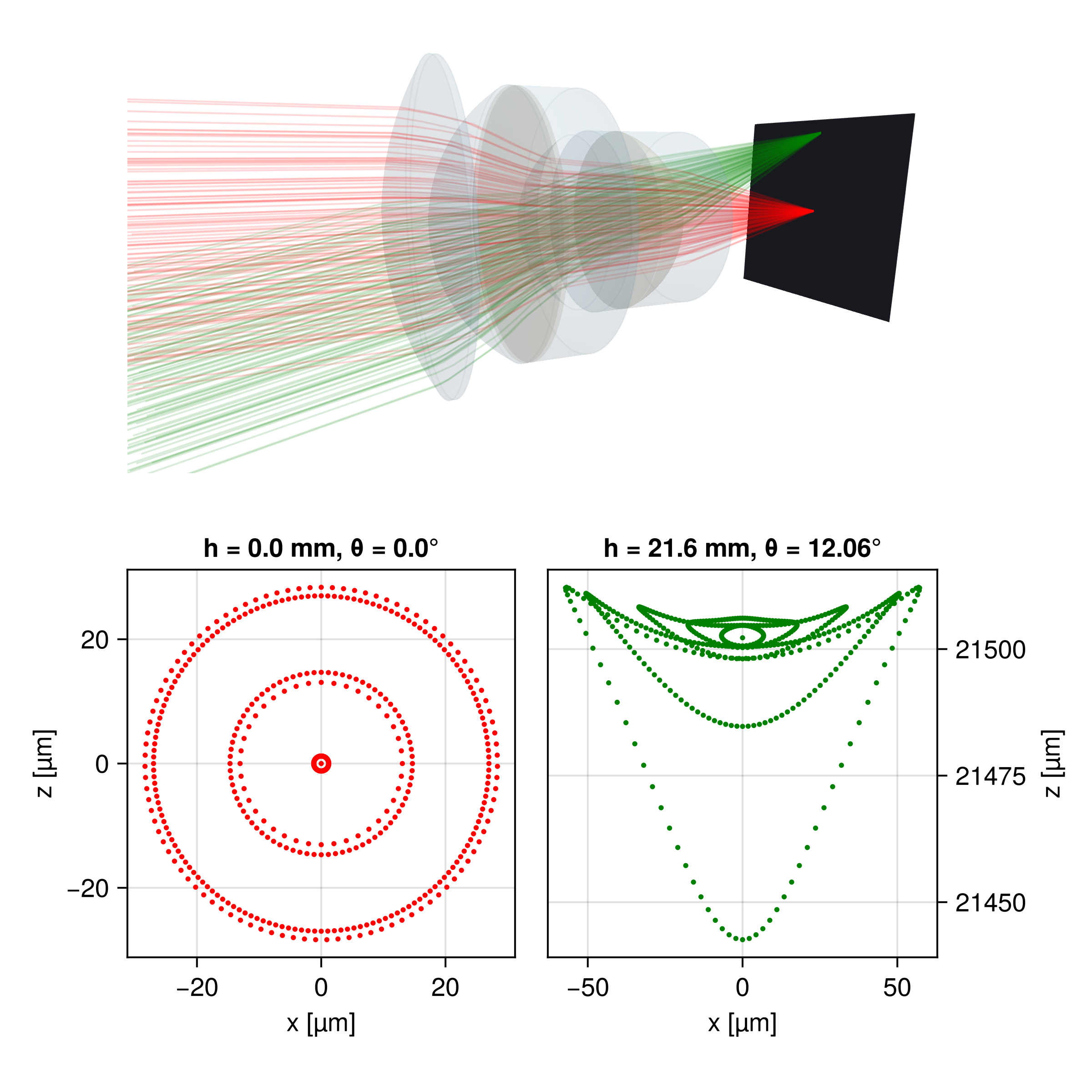
source

The following image shows the spot diagram of a Sonnar lens. Two CollimatedSources are traced through the system at different angles. A Detector is positioned at the focal plane to capture the resulting spot diagrams, which are visualized using the method explained above.

Ray directions

Where a ray crossed the detector is half of what it carries; ray_hits also returns the direction in which it went, both in the coordinates of the detector. The angle of each ray to the detector normal over its distance from the detector center shows, for example, how far a beam is from collimated:

using LinearAlgebra: norm
pts, dirs = ray_hits(pd)
r = norm.(pts)                                   # distance from the detector center [m]
θ = [atan(hypot(d[1], d[3]), abs(d[2])) for d in dirs] # angle to the normal [rad], either side

BeamletOptics.ray_hits Function

ray_hits(pd::Detector) -> (points, directions)

Where each ray crossed the Detector pd and in which direction it went, in the coordinates of the detector. points[i] is the local (x, z) of hit i in [m], as in spot_diagram, and directions[i] its unit direction in the right-handed frame (x̂, n̂, ẑ), with the local axes x̂, ẑ and the normal n̂ = -direction(pd), along which beams arrive on the front side. For a detector in its initial orientation this frame is the global one, so a beam along the optical axis has the direction (0, 1, 0). A hit on the back side, which the detector also records, has d[2] < 0. The angle of a ray to the detector normal, in [0, π/2] for either side, is atan(hypot(d[1], d[3]), abs(d[2])) (accurate also near 0, unlike acos), its distance from the detector center norm(p), e.g. to judge how far a beam is from collimated.

For GaussianBeamlets and AstigmaticGaussianBeamlets, each hit gives the point and direction of the chief ray of the beamlet, whereas spot_diagram gives its waist contour. The pairs follow the order of the stored hits, which is not deterministic for beam groups. A detector that no beam hit returns two empty vectors.

source

Field distributions

Alternatively, the detector data can also be used to reconstruct electric field distributions of incoming beams on its surface using coherent addition. Three readouts build on each other: electric_field is the coherent sum of the fields of all hits, intensity the flux of the Poynting vector of that field through the detector, and optical_power the integral of the intensity. Their definitions follow.

BeamletOptics.electric_field Method

electric_field(pd::Detector, sampling::AbstractDetectorSampling = RegularGrid(); progress = true)

Samples the electric field of the hits of the Detector pd at the points of sampling in its local (x, z) plane, by default a RegularGrid in a window around the hits. The field at the local point (x, z) is the coherent sum of the fields Eⱼ of all hits j,

with the position p_d of the detector and its local axes x̂, ẑ, which form a left-handed system with the detector normal. Eⱼ is defined per hit type in electric_field(::BeamletOptics.AbstractDetectorHit, ::AbstractVector). The field is not projected onto the detector: it is the field that is there, for any angle of incidence. The power per detector area follows from intensity, which takes the angle of incidence of each hit into account. To sample on a grid of one's own, pass a RectilinearGrid; other samplings are subtypes of BeamletOptics.AbstractDetectorSampling.

Coherent sum

All hits are summed as one monochromatic, mutually coherent field, also hits of different wavelengths or of sources that are mutually incoherent. For those, evaluate the intensity of each wavelength or source on its own and add the intensities.

Resetting detectors

Be sure to call empty!(pd) (or initialize!(system) for all detectors) before each new measurement if reusing the same detector.

Keyword arguments

• progress::Bool = true: shows a progress bar once the calculation has run for get_progress_threshold() seconds (default 5 s). It is only drawn if stderr is a terminal.

The grid, its window and its resolution are set by the sampling, e.g. electric_field(pd, RegularGrid(num_points = 200, crop_factor = 5)), see RegularGrid.

Scaling

The returned values for ray hits correspond to the E-field of the point spread function. The values are raw/unscaled and not equal to a Strehl ratio: a Ray has the amplitude 1, a PolarizedRay its field vector E0, which carries the Fresnel/Jones amplitude factors but not the ray-tube area or the pupil sampling density.

Returns

The coordinates of the sampling followed by the field at its points, for the grids (xs, zs, E) with E[i, j] at (xs[i], zs[j]), see sample_points. The values are complex scalars for Rays and GaussianBeamlets, Point3{Complex{T}} 3D vectors in global coordinates for PolarizedRays and AstigmaticGaussianBeamlets, which carry a polarization. A detector that no beam hit has the field zero at every point, as complex scalars, since without hits there is no polarization.

Unpolarized light

An unpolarized PSF is not obtained from a single coherent trace. Instead, trace twice with orthogonal input polarizations (e.g. E0 = [1,0,0] and E0 = [0,0,1]), evaluate intensity(pd, sampling) with the same RectilinearGrid sampling after each trace and add the results.

source

BeamletOptics.electric_field Method

electric_field(hit::AbstractDetectorHit, p::AbstractVector)

Electric field Eⱼ(p) of a single detector hit at the global point p [m], not projected onto the detector: a complex scalar for RayHits and GaussianBeamletHits, a complex 3D vector in global coordinates for PolarizedRayHits and AstigmaticGaussianBeamletHits. It is a phasor with the time dependence exp(-iωt), so that a plane wave in a medium of index n carries the intensity n|E|²/(2Z₀). With the vacuum wavenumber k₀ = 2π/λ, the direction s of the hit, the refractive index n in front of the detector and the optical path length L from the source to the hit point p_hit:

• RayHit: a plane wave of amplitude 1,

• PolarizedRayHit: the same plane wave times the field vector E₀ of the ray,      

• GaussianBeamletHit: the TEM₀₀ field of the traced segment, at the distance l along its chief ray and the distance r from it,

  with the field E₀ and waist w₀ of the beamlet, the beam radius w, the radius of curvature R and the Gouy phase ψ of the segment (see gauss_parameters), the index n of the segment and the optical path L(l) along the chief ray.

• AstigmaticGaussianBeamletHit: the field vector of the chief ray of the segment, E₀, times the general astigmatic Gaussian beam of its parabasal rays,      , with the Gouy factor g, which also holds the change of the amplitude with the beam area, the transverse phase W, the spot matrix S at the offset r from the chief ray and κ = det S / |a|² of the complex beam area a, see Astigmatic polarized beamlets.

Beamlet hits give the physical field in [V/m]. Ray hits are raw and unscaled: |E|² does not carry the power of the ray, see the note on scaling in electric_field(pd, sampling).

A new hit type implements this method and the other functions listed in BeamletOptics.AbstractDetectorHit; the readouts of a Detector on a grid (electric_field, intensity, optical_power) then work for it.

source

BeamletOptics.intensity Method

intensity(pd::Detector, sampling::AbstractDetectorSampling = RegularGrid(); progress = true)

Samples the irradiance on the Detector pd, the power per detector area in [W/m²], at the points of sampling, by default a RegularGrid around the hits. Returns the coordinates of the sampling followed by the irradiance at its points, for the grids (xs, zs, I); progress as for electric_field(pd, sampling).

I is the flux of the coherent sum of all hits through the detector: the time-averaged Poynting vector along the detector normal n̂, which points along the incoming beams. Hits with a polarization (PolarizedRays, AstigmaticGaussianBeamlets) give

with the field Eⱼ of hit j (see electric_field(hit, p)), its direction sⱼ, the refractive index nⱼ in front of the detector, the vacuum impedance Z₀ and σⱼ = sign(sⱼ ⋅ n̂), i.e. a hit on the back side of the detector counts like one on its front side. Hits without a polarization (Rays, GaussianBeamlets) have no vector H and give the scalar form of the same flux,

A single hit under the angle θ to the normal gives I = n|E|² cos θ / (2Z₀), the power of the beam per detector area, so that optical_power is the power of the beam for any angle of incidence. No projection factor is applied to the field. For two scalar hits, the cross term is Re(E₁* E₂) (n₁ cos θ₁ + n₂ cos θ₂) / (2Z₀), i.e. hits under different angles interfere with the mean of their n cos θ.

I is in [W/m²] for beamlet hits. For ray hits, whose fields are unscaled, it has the same form but no absolute unit. A detector that no beam hit has I = 0 at every point.

source

BeamletOptics.optical_power Method

optical_power(pd::Detector, sampling::AbstractDetectorSampling = RegularGrid(); progress = true)

Calculates the total optical power on pd in [W] as the integral of its intensity over the window of sampling in the local detector coordinates,

with the points (xᵢ, zᵢ) and the weights wᵢ [m²] of the sampling, see sample_points: the trapezoidal rule for RegularGrid and RectilinearGrid. Since I is the flux through the detector, P is the power of the beams for any angle of incidence.

The integral runs over the window of the sampling, not over the active area of the detector: the window is not cut at the edges of the detector. The default window of beamlet hits holds the power of each beamlet except for a part of 10⁻⁸, see crop_factor of RegularGrid. For ray hits, P has no absolute unit, see intensity. A detector that no beam hit gives P = 0, e.g. when a scan moves the beam off the detector.

source

Sampling

Where on the detector the readouts are evaluated is set by a sampling, the second argument of each readout. It chooses its window, the points in local detector coordinates and the weights with which optical_power integrates the intensity. The default is a RegularGrid around the hits; a RectilinearGrid is a grid of one's own with any spacing.

x, z, I = intensity(pd, RegularGrid(num_points = 200, crop_factor = 5))
P = optical_power(pd, RectilinearGrid(xs, zs))

The steps of a readout and the methods a new sampling or hit type implements are shown in Readout pipeline.

BeamletOptics.RegularGrid Type

RegularGrid(; num_points = 100, center = Centroid(), crop_factor, x_min, x_max, z_min,
    z_max, x0_shift = 0, z0_shift = 0)

The default sampling of a Detector: num_points×num_points equidistant points in a window around its hits, in local detector coordinates. The readouts return (xs, zs, values) with values[i, j] at (xs[i], zs[j]); optical_power integrates with the trapezoidal rule. The window follows from the hits when the readout is evaluated, see calc_local_lims. A detector that no beam hit has the window of its active surface.

Keyword arguments

• num_points::Int = 100: number of points per axis.

• center::AbstractCenterAlgorithm = Centroid(): for ray hits, how the window is centred: Centroid() uses the projection-weighted centroid, MinMax() the mid-point of the bounding box.

• crop_factor::Real: scales the width of the window around the hits; values >1 expand, <1 shrink. The default is 1 for ray hits (the box around the hit points) and 3 for beamlet hits (three beam radii around each hit, which holds the power of a Gaussian beam except for a part of 10⁻⁸).

• x_min, x_max, z_min, z_max: bounds of the window in [m]. A given bound replaces its side of the window around the hits, the others stay automatic. If a lower bound ends up above its upper one, the readout throws an ArgumentError.

• x0_shift = 0, z0_shift = 0: shift the whole window along x or z in [m].

source

BeamletOptics.RectilinearGrid Type

RectilinearGrid(xs::AbstractVector, zs::AbstractVector)

A Detector sampling on the grid xs × zs of local detector coordinates in [m], with any spacing: the readouts return (xs, zs, values) with values[i, j] at (xs[i], zs[j]). optical_power integrates with the trapezoidal rule along both axes. The window is xs × zs as given, independent of the hits. Both axes must be non-empty and ascending, otherwise an ArgumentError is thrown: a descending axis would integrate to a negative power.

source

BeamletOptics.electric_field Method

electric_field(pd::Detector, points::AbstractArray{<:AbstractVector}; progress = true)

The field of the hits of the Detector pd at the local detector coordinates points in [m], an array of vectors (x, z) (e.g. Point2s), see electric_field(pd, sampling). Returns the values only, in the shape of points.

source

BeamletOptics.intensity Method

intensity(pd::Detector, points::AbstractArray{<:AbstractVector}; progress = true)

The irradiance on the Detector pd in [W/m²] at the local detector coordinates points in [m], an array of vectors (x, z) (e.g. Point2s), see intensity(pd, sampling). Returns the values only, in the shape of points.

source

Gaussian beamlet interference

One of the use cases of the Detector is to analyse interference patterns. Below a rendered example of a detector model (FDS010) can be seen. The detector active area is marked in blue (1x1 mm²).

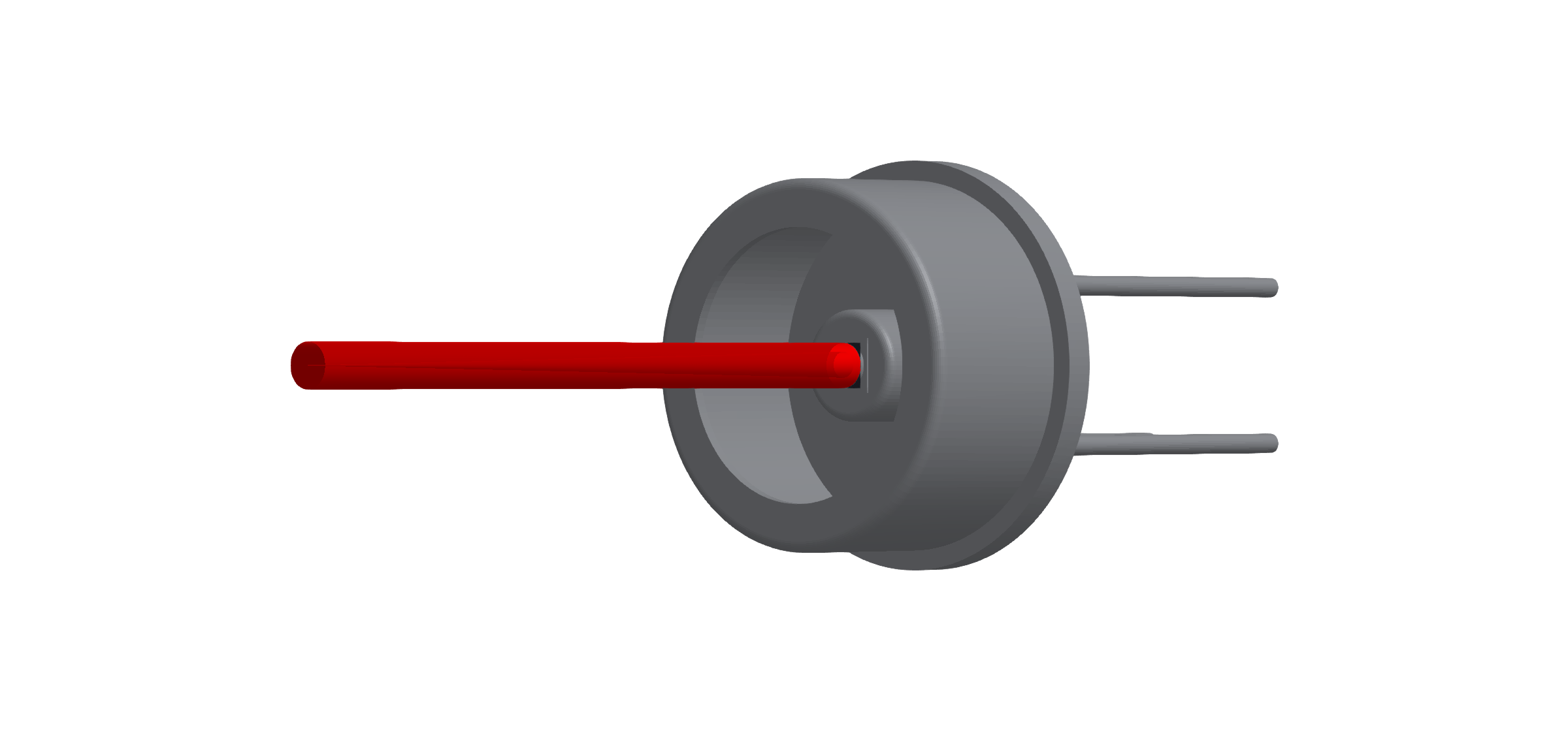
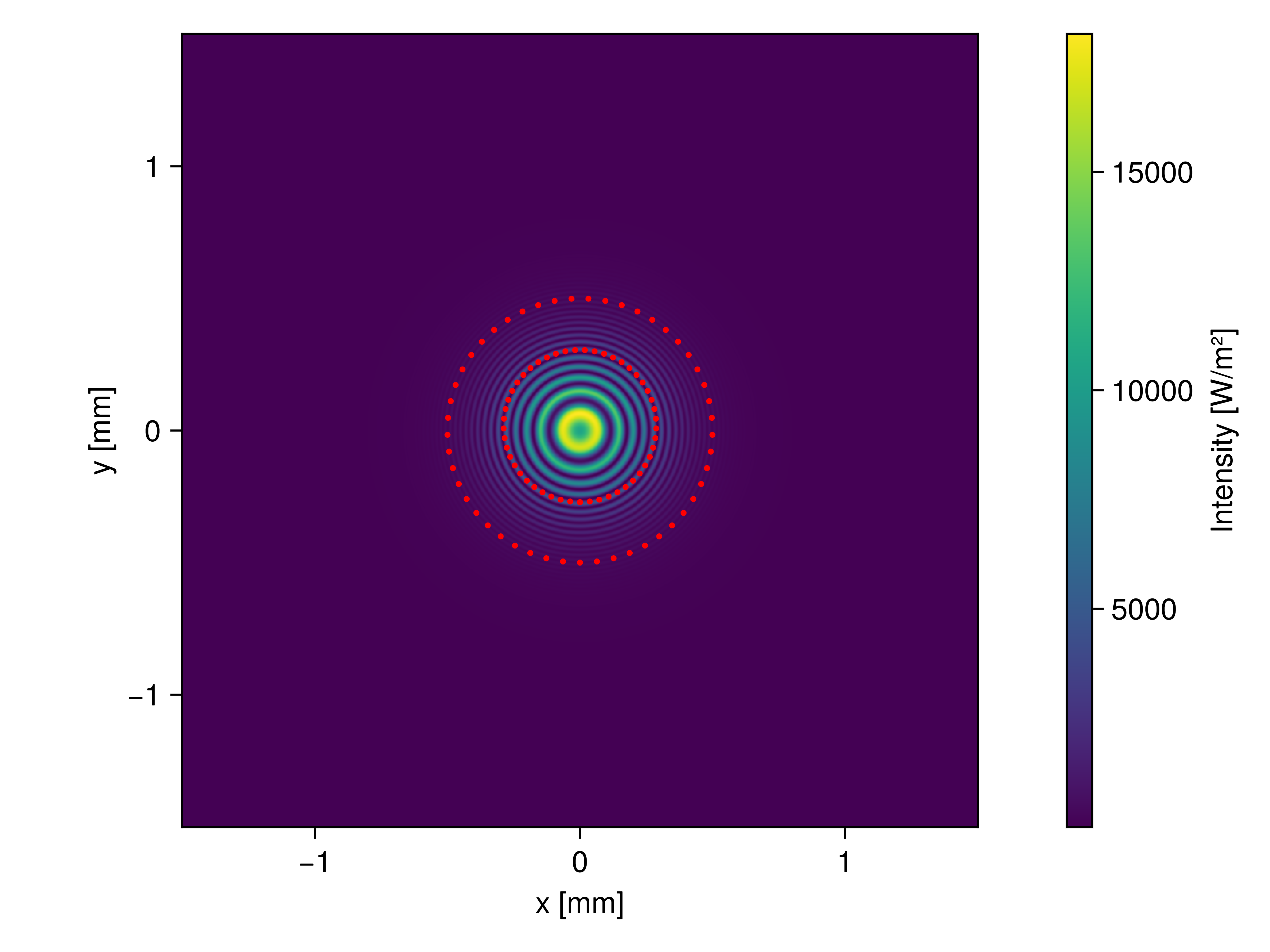
The figure below demonstrates an example intensity distribution captured by the detector pictured above, showing radial fringes due to a mismatch of the radii of curvature of the interfering GaussianBeamlets. In addition, the beam waists have been visualized.

Interferometer tutorial

Refer to the Michelson interferometer section for a detailed tutorial on how to use the Detector.

Point spread function estimation

If a Detector is placed in the focal plane of an imaging system, the coherent addition of the ray-attached plane waves yields an estimate of its point spread function (PSF). For the Sonnar example from the Spot diagrams section the following distribution was calculated for the on-axis beam bundle.

Experimental feature

The PSF estimation does not use pupils (yet) but merely superimposes the ray-attached plane waves. It gives qualitatively sound results, but requires good sampling of the problem to be quantitatively meaningful. No Strehl ratio is calculated.

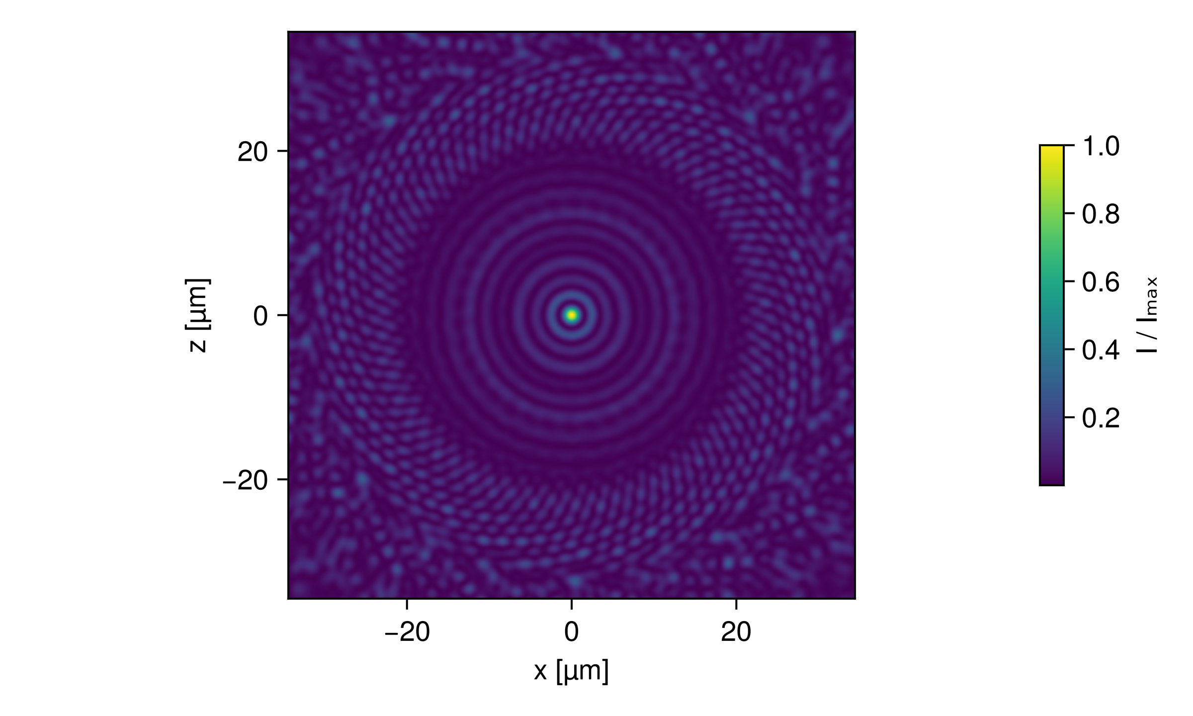
For PolarizedRays the field is added as 3D vectors, so electric_field returns a matrix of complex vectors and each component of the focal field can be analyzed separately. This becomes relevant at high NA, where the field vectors tilt towards the optical axis. The same holds for AstigmaticGaussianBeamlets.

PSF examples

The Point spread functions example page covers the Airy disc, an aberrated asphere and the vectorial focus of a parabolic mirror at NA 0.88, including the caveats on collimated sources and ray amplitudes.

OpticsBase interoperability

If OpticsBase.jl is loaded alongside BMO (using OpticsBase), the BeamletOpticsOpticsBaseExt package extension adds a PlaneField constructor for a Detector. It samples the physical field of the beamlet hits as tangential electric and magnetic field on the detector plane, OpticsBase's single exchange format for coupling to other Maxwell solvers (angular spectrum propagators, BPM, FDTD, ...). As for intensity(::Detector), the Poynting flux of an oblique beam through the plane is the full beam power.

The field is built from the hits as follows:

• E is the coherent sum of the 3D fields of the hits at the sample points, projected onto the plane axes and .

• H is the coherent sum, over hits, of   . Here is the propagation direction of the chief or stigmatic ray of hit and is that hit's own 3D field contribution at the sample point. It is not the paraxial    built from the total field, which would be exact only for normal incidence. This matches the surface-equivalence-theorem content of PlaneField even for beams that hit the plane off-normal.

• The default axes follow the detector: is -direction(detector) (BMO's detector normal points against the beam, so points downstream, the direction the light was travelling in when it hit the detector), is the local detector x axis of BMO and    is BMO's local axis. This is the default port of BMO's detector readouts.

• AstigmaticGaussianBeamletHits carry the polarization of their chief ray, so their field is electric_field(hit, p) already. A stigmatic GaussianBeamletHit carries no polarization in BMO (the model is scalar). By convention, matching OpticsBase's own rule for a scalar field (PlaneField(E::AbstractMatrix, ...) puts a scalar field entirely into Eu), its contribution is polarized along the plane's axis, made transverse to the hit direction (along if is parallel to it), so that   and     form a consistent plane wave. At normal incidence this is exactly .

• R = Inf: no reference sphere is removed, because BMO's beamlet field already carries the full spatial phase without needing one.

The internal steps of these constructors are shown in OpticsBase extension internals.

OpticsBase.PlaneField Method

OpticsBase.PlaneField(detector::BeamletOptics.Detector;
    size::NTuple{2,Int}, spacing::NTuple{2,Real},
    origin = BeamletOptics.position(detector), axes = <default detector frame, see below>,
    progress = true)

Samples the coherent field of the beamlets hitting a BeamletOptics (BMO) Detector into an OpticsBase.PlaneField. Call it after solve_system!. The hits keep the state of their solve: solving again or moving other objects does not change them, moving the detector empties it. Requires using OpticsBase (package extension).

Arguments

• detector: a BMO Detector whose hits are all GaussianBeamletHit or all AstigmaticGaussianBeamletHit (i.e. Gaussian beamlet sources). All hits must share the vacuum wavelength and the refractive index of the medium in front of the detector.

• size (keyword, required): number of samples (nx, ny) along the plane's u, v axes.

• spacing (keyword, required): sample spacings (Δu, Δv) in [m], as in OpticsBase.PlaneField.

• origin (keyword): center of the plane in global coordinates in [m]. Default: the detector position.

• axes (keyword): 3×3 matrix with columns u, v, n (see OpticsBase.PlaneField). Default: n = −direction(detector) (downstream, the direction of the light that hit the detector), u the local detector x axis of BMO and v = n × u, the default port of BMO's detector readouts.

• progress (keyword): show a progress bar. Default: true.

Conventions

• E is the physical field: the coherent sum of the beamlet fields at the plane's sample points, projected onto u, v. Like electric_field(detector), it carries no projection factor; for oblique beams power(f) is the full beam power crossing the plane, as optical_power(detector).

• H is the coherent sum over hits of (n_medium/Z₀) dᵢ × Eᵢ, with dᵢ the propagation direction of the chief/stigmatic ray of hit i and Eᵢ that hit's own 3D field at the sample point.

• R = Inf: no reference sphere is removed.

• Eᵢ is the 3D field of each hit: AstigmaticGaussianBeamletHits carry the polarization of their chief ray, Eᵢ is their field vector (electric_field(hit, p)). A stigmatic GaussianBeamletHit (scalar model) is polarized along the plane's u axis made transverse to the hit direction (along v if u is parallel to it). At normal incidence this is exactly u.

• n (medium refractive index) is that of the hits; λ is their shared wavelength.

• Time convention exp(−iωt), as in BMO and OpticsBase.

Throws an ArgumentError if the detector has no hits, since a PlaneField takes λ and n from them, if the hits are not beamlet hits (e.g. ray hits), or if they do not share wavelength and refractive index.

source

The return paths, WavefrontBeamletDecomposition and GaussianModeDecomposition for a PlaneField, are documented in OpticsBase fields as beam groups. Without a detector, a single traced beamlet segment is sampled with PlaneField(beamlet, id; ...), which components that hand light to another solver use in their interact3d method, see Re-emitting components.